This project explores the use of homographies to warp images to different perspectives and create photo mosaics. Part B follows the paper Multi-Image Matching using Multi-Scale Oriented Patches to automate the stitching process.
To compute the matrix H describing a particular homography between a set of n pairs of points, I use least squares to solve the below linear system b = Ax for x, where x is a vector with the 8 free values of H, and b and A are defined as below, with two rows for each correspondence.
With a computed inverse transformation matrix, I implemented inverse warping to apply transformations to images.
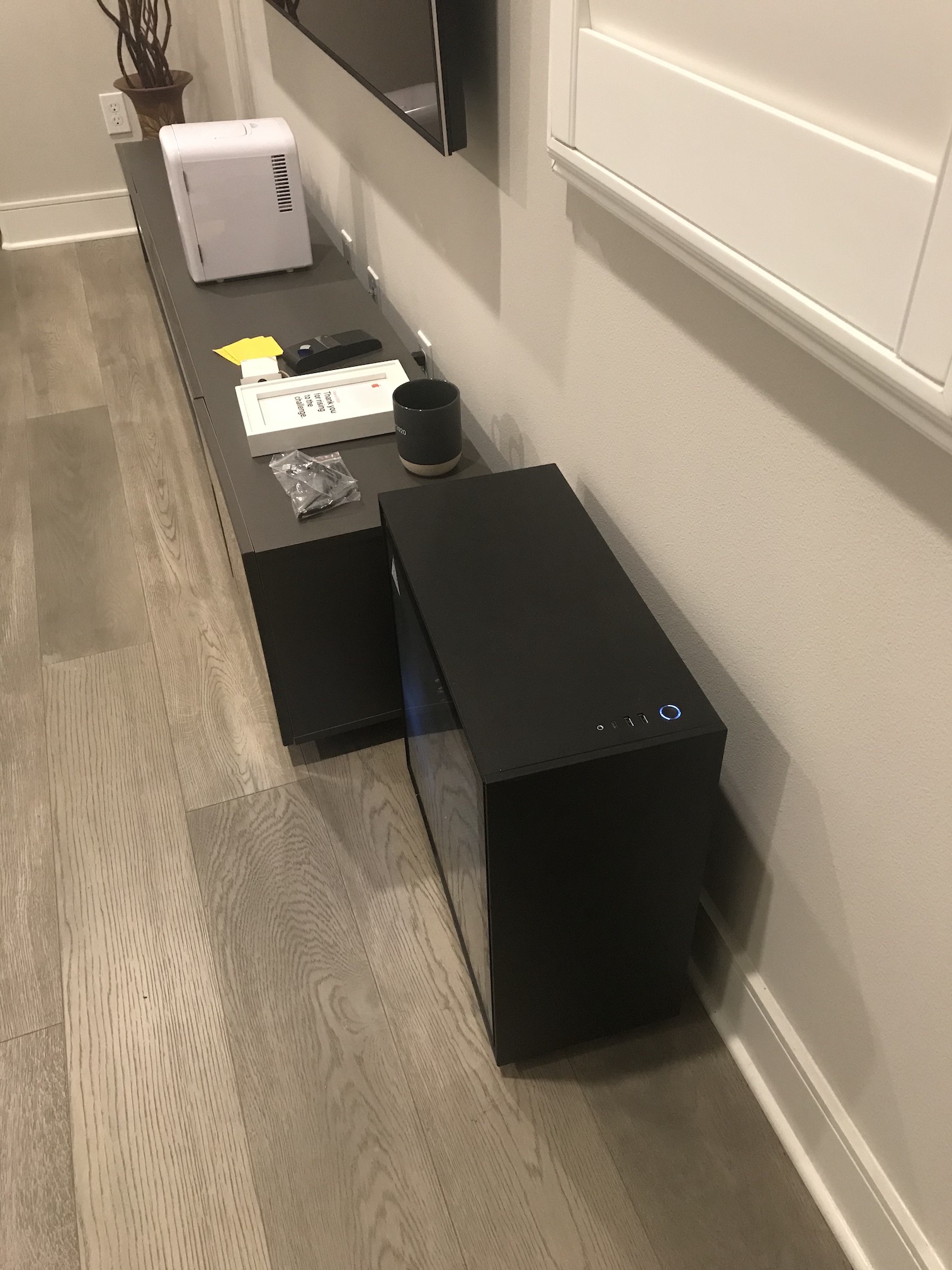
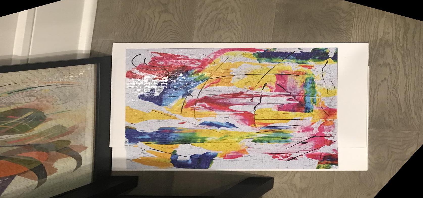
I took an image of the below computer and rectified the top surface using the warping function implemented in the previous section (mapping the corners of the top surface to a rectangle).
| Original | Rectified (Cropped) |
|
|
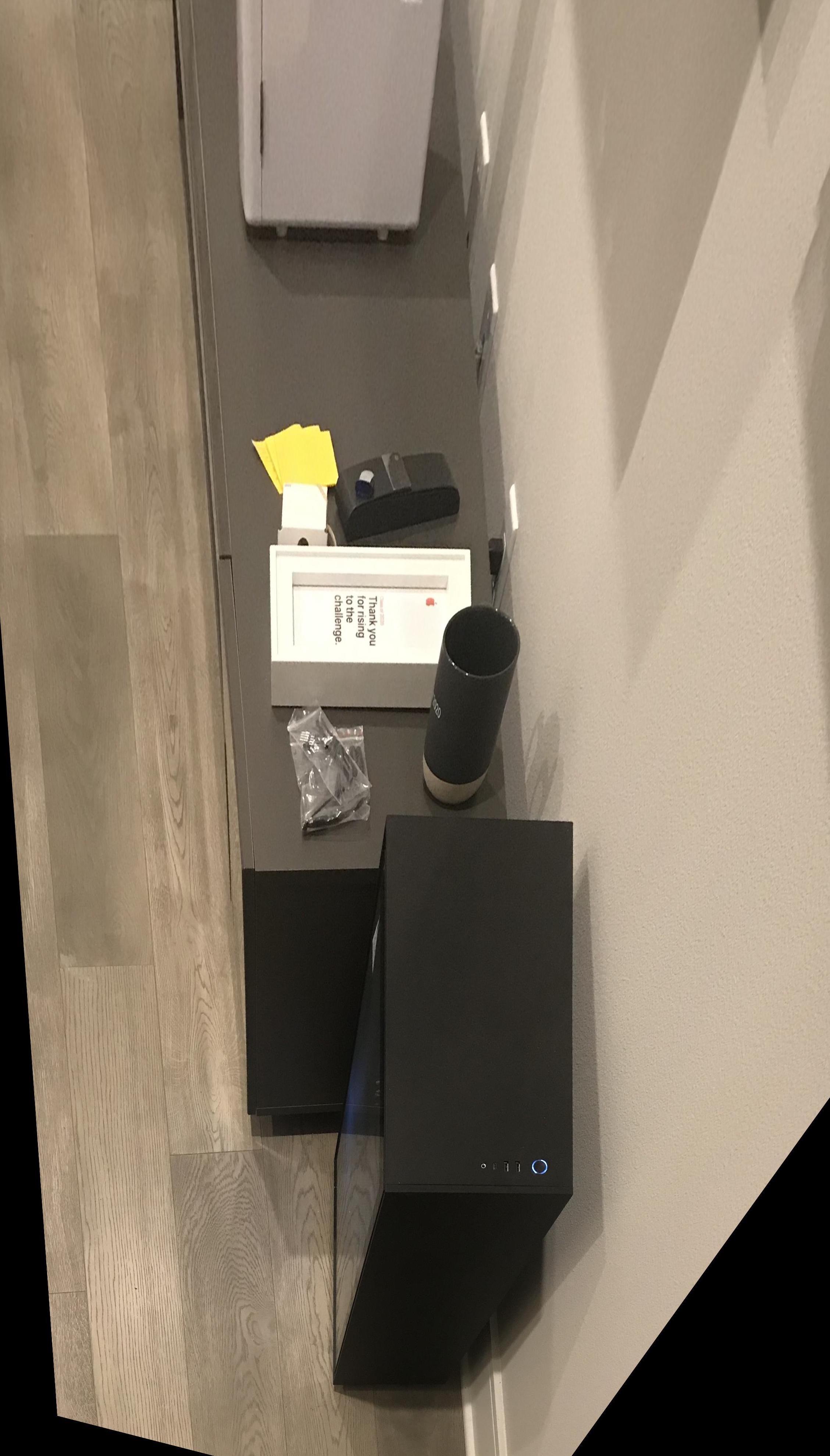
Here's another example:
| Original | Rectified (Cropped) |
 |
 |
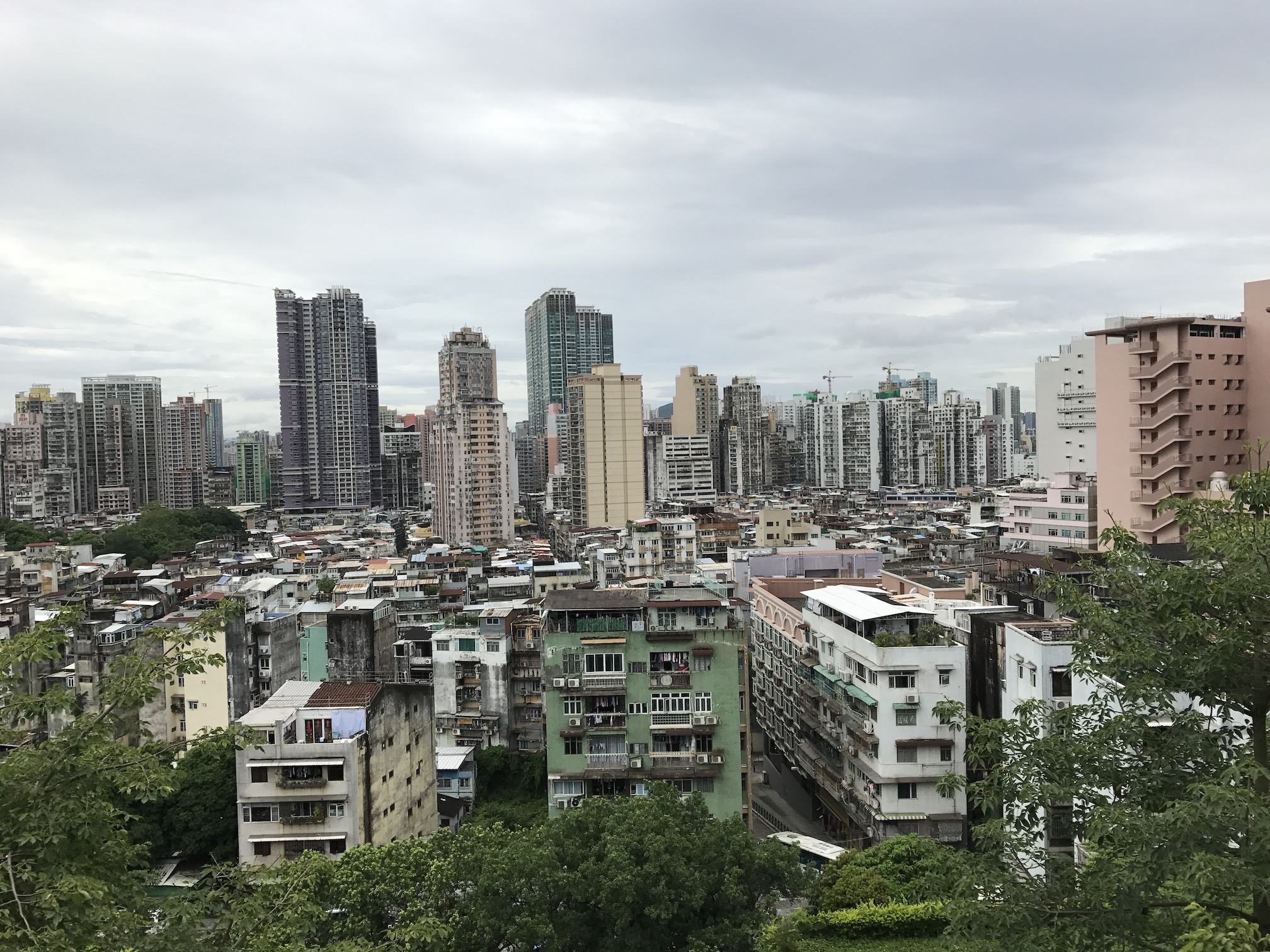
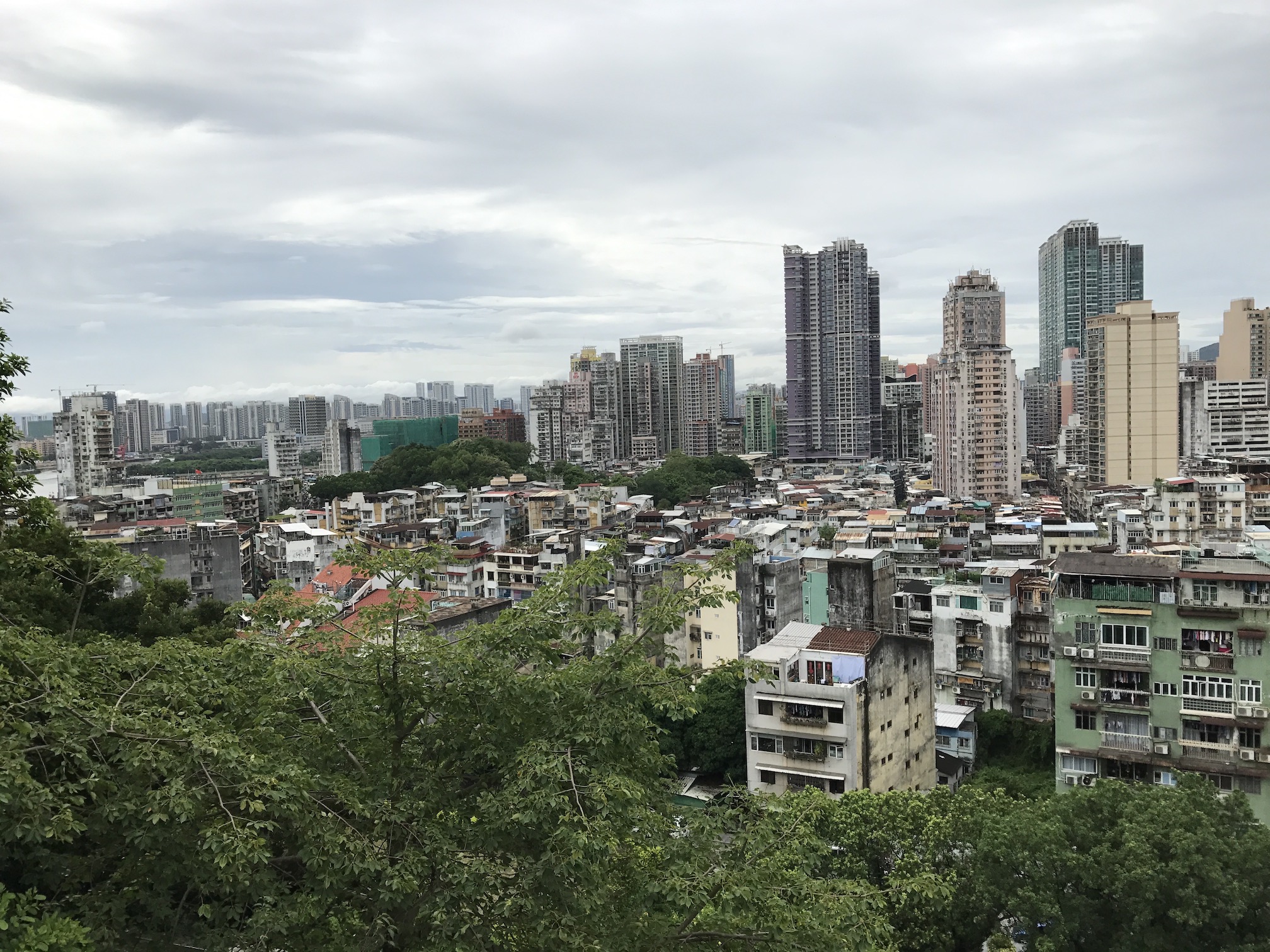
I pulled a couple old images off my camera roll, and downsampled them to a reasonable resolution for this part. To stitch the images together, I manually defined 10 corresponding points in each image to be used for the homography:
| Original im1 | Original im2 |
 |
 |
| Selected Points for im1 | Selected Points for im2 |
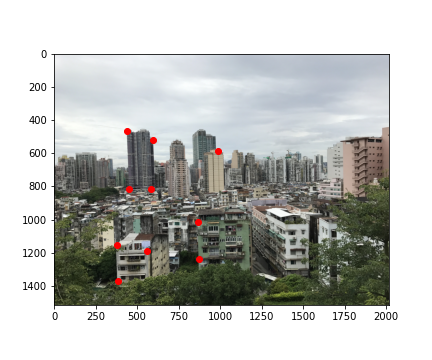 |
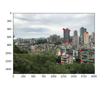 |
My stitching process was as follows:
For this project, for the mask, I assigned each unwarped image an alpha channel. I ended up just using a gaussian multiplied by a mask that linearly falls off to 0 at the edges. Below are the results from this procedure.
| Blended Result |
 |
| Original im1 | Original im2 |
 |
 |
| Blended Result |
 |
| Original im1 | Original im2 | Original im3 |
 |
 |
 |
| Blended Result (first 2 images) |
 |
I enjoyed learning about recovering homographies for a set of corresponding points, and translating the linear algrebra discussed in lecture to python code for this project. I experimented the most with the mosaicing section, however. I initially did a simple averaging for the overlapping region to blend the images, but I wasn't satisfied with the sharp edges and the overlapping high-frequencies in my results. I added the radial alpha to address the first issue, then re-used the Project 2 code to address the second. While my final image is better, there are still some areas where the blending isn't perfect (e.g. the front of the white house in the center foreground could be clearer).
I used the provided harris.py to find potential corners and h-values. There are many; I display the top 500 for each image below:
| First 500 Harris corners for im1 | First 500 Harris corners for im2 |
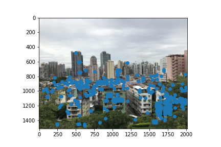 |
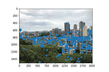 |
I implemented ANMS as described in the paper to achieve a more even distribution of corners, computing the r-value for each coordinate and selecting the coordinates with the smallest values. I used the same value of c_robust = 0.9 as used in the paper, and use ANMS to get the top 500 coordinates:
| ANMS (n=500) for im1 | ANMS (n=500) for im2 |
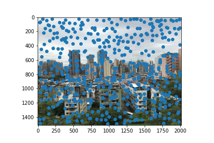 |
 |
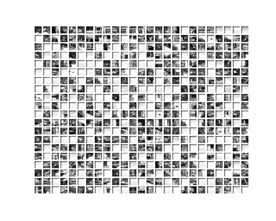
For the 500 corners selected with ANMS, I implemeted a simpler feature descriptor than the one described in the paper. Specifically, for each corner, I do the following:
This does not implement the rotation-invariance or the wavelet transformation described in the paper. Here are the 500 feature descriptors for im1, visualized.
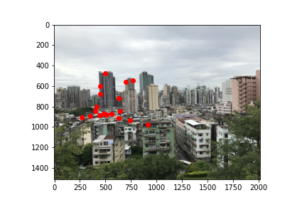
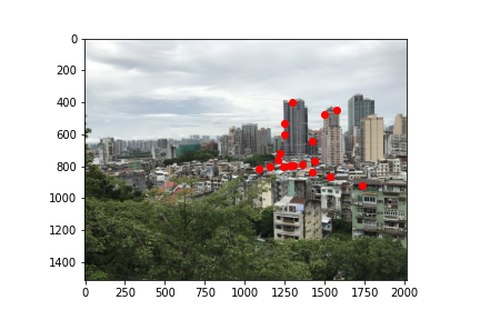
For feature matching, I used the simple Lowe approach with a threshold of 0.2. For each patch of a particular image, this involves taking the ratio of the l2 distance of the 1-nearest neighboring patch and the 2-nearest neighboring patch of the other images, and checking if that ratio is below the thresold value. Below are the results of this approach on my images:
| Matched corners on im1 | Matched corners on im2 |
 |
 |
I implemented 4-point RANSAC as described in lecture to compute a robust homography for the matched features. This involves repeatedly taking random samples of 4 matching points and computing a set of "inliers" (e.g. points that map to a position within some error eps of the matched position). The largest set of inliers can be used to compute the final homography between the points. I ran this for 100 iterations and with an eps=1.0.
The homography produced by RANSAC can then be passed into the stitching method created in Part A to blend the images together.
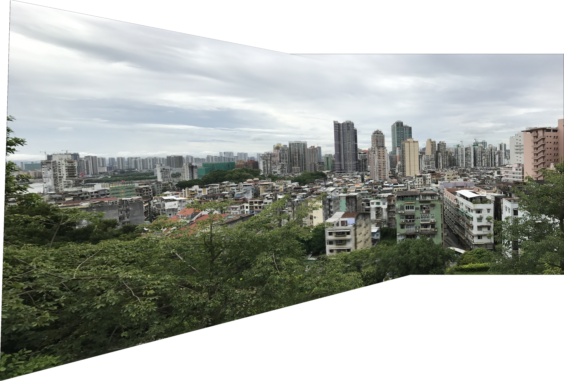
Below are results comparing the manually-matched mosaics with the auto-stitched mosaics:
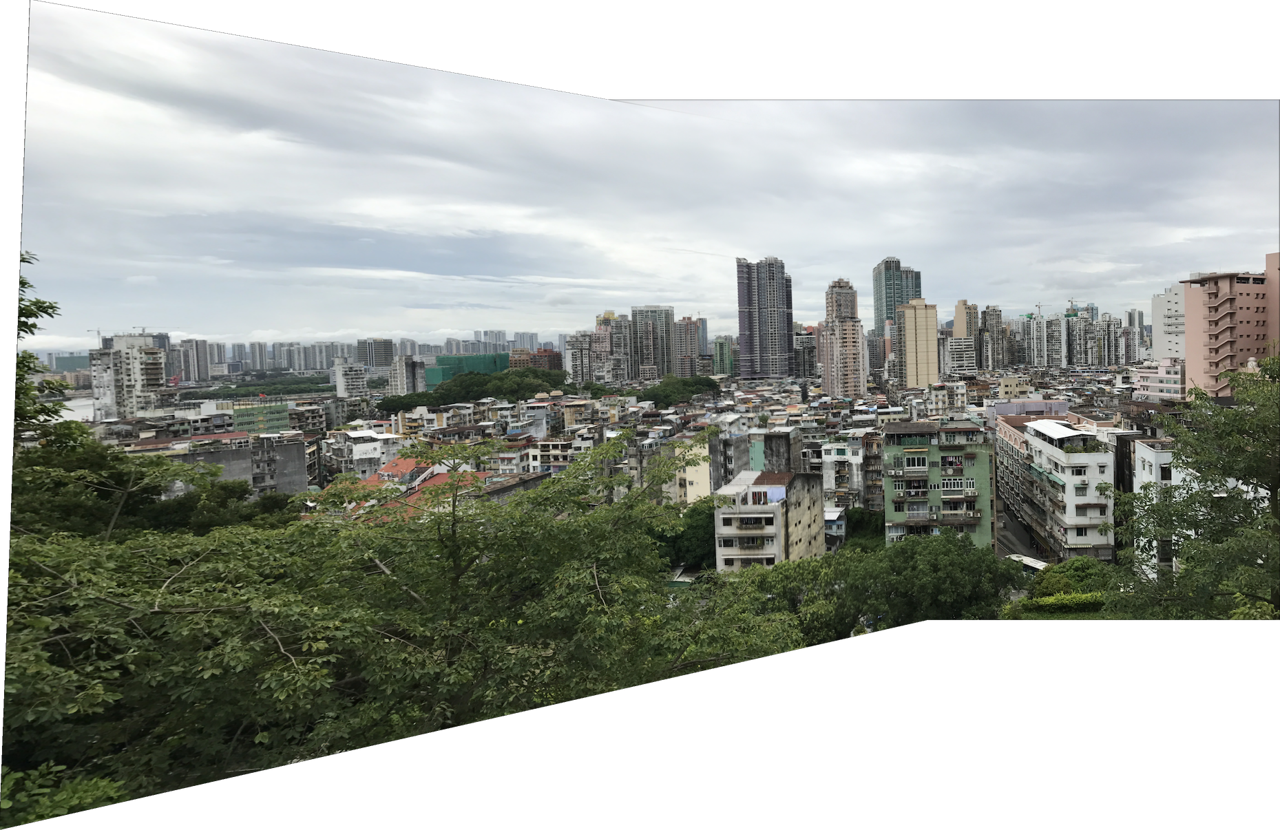
| Manual Mosaic - Macau |
|
| Autostitched Mosaic - Macau |
 |
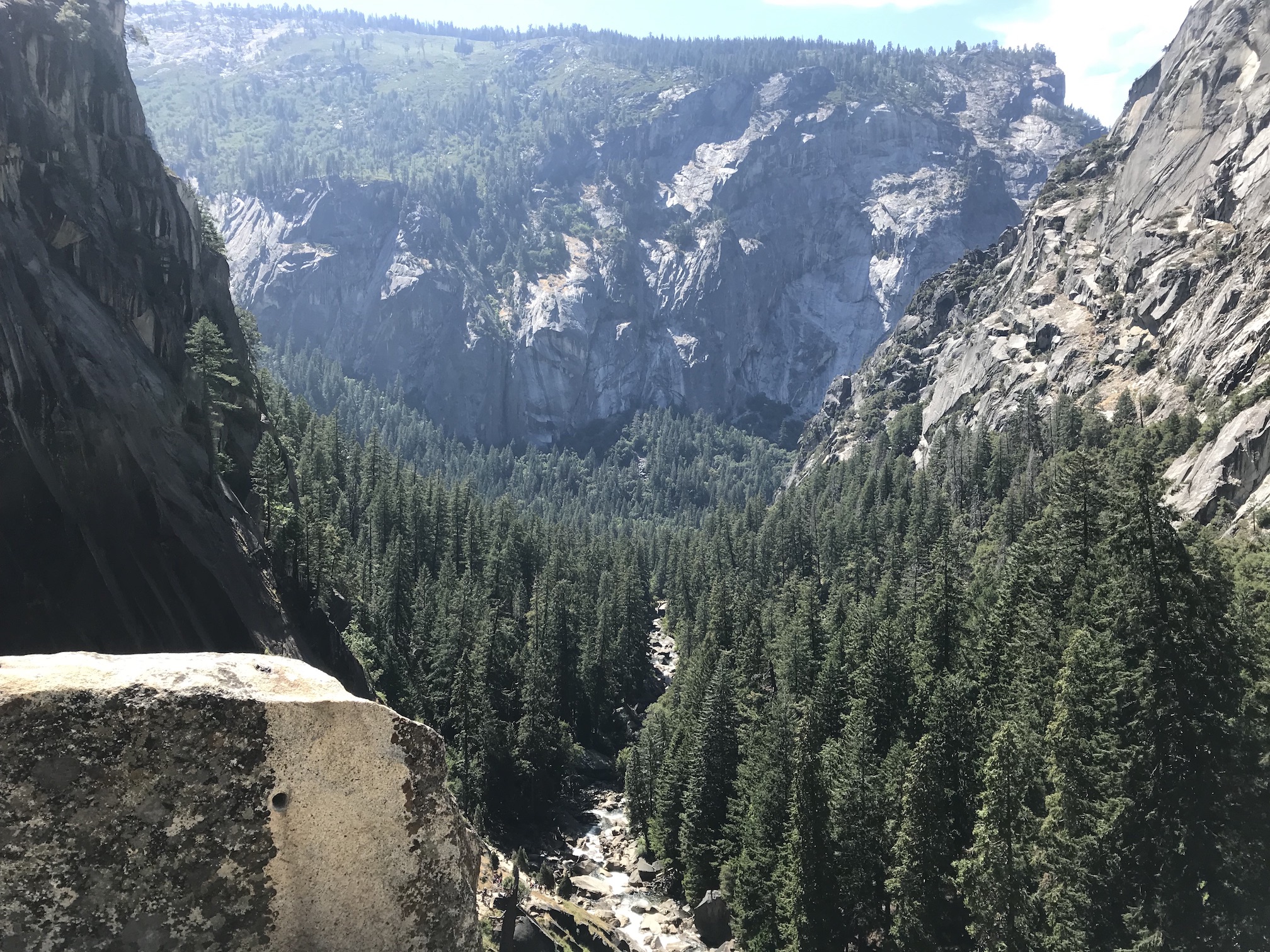
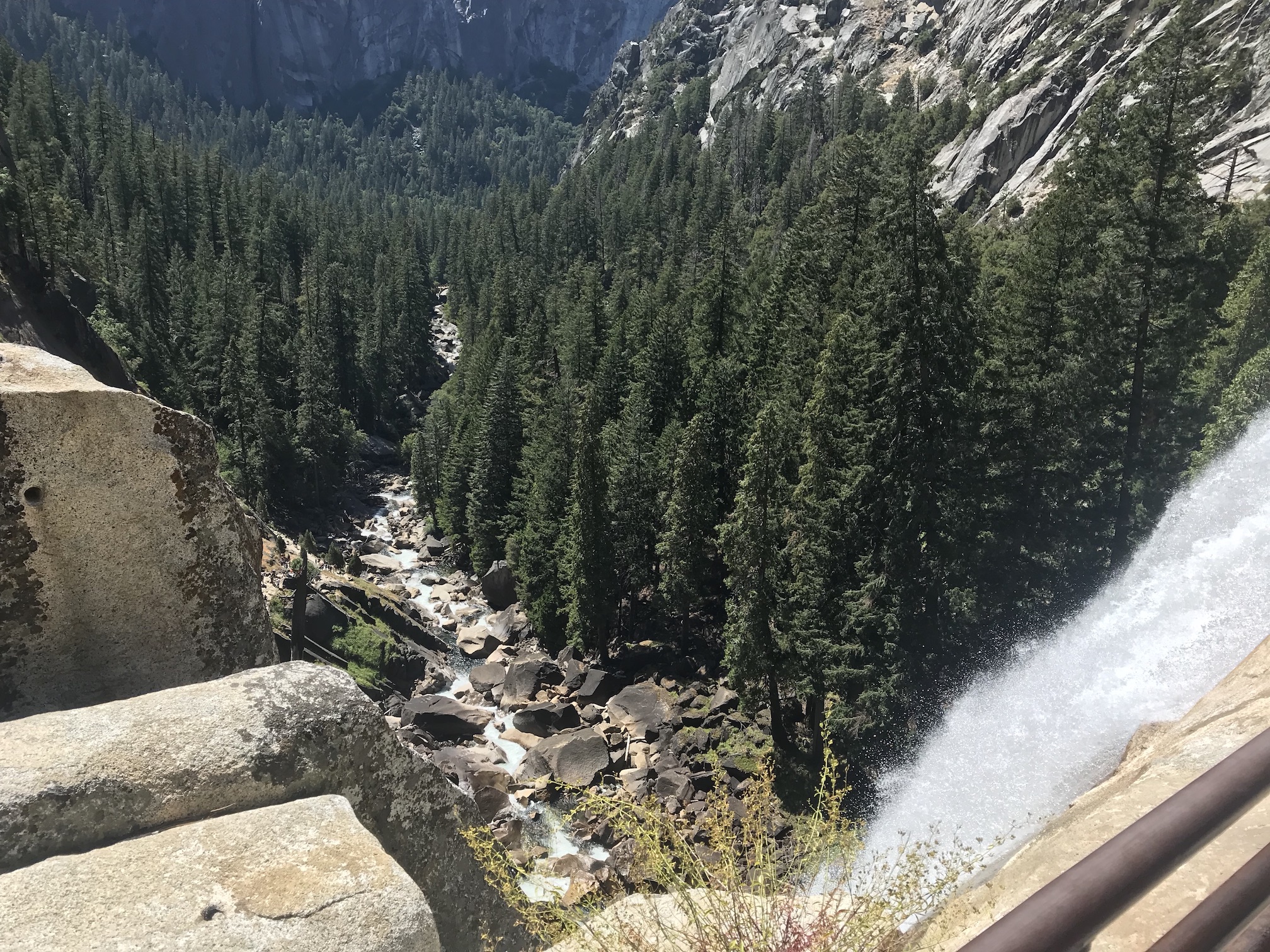
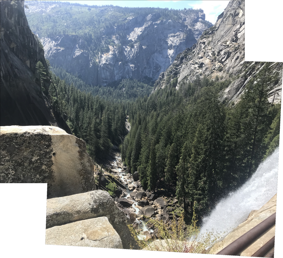
| Manual Mosaic - Yosemite |
|
| Autostitched Mosaic - Yosemite |
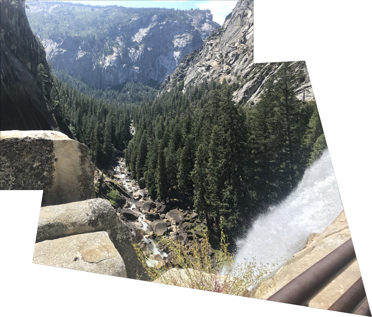 |
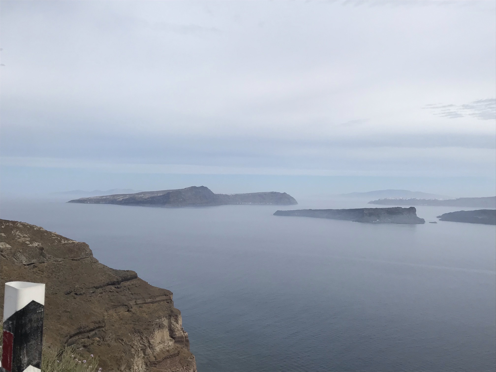
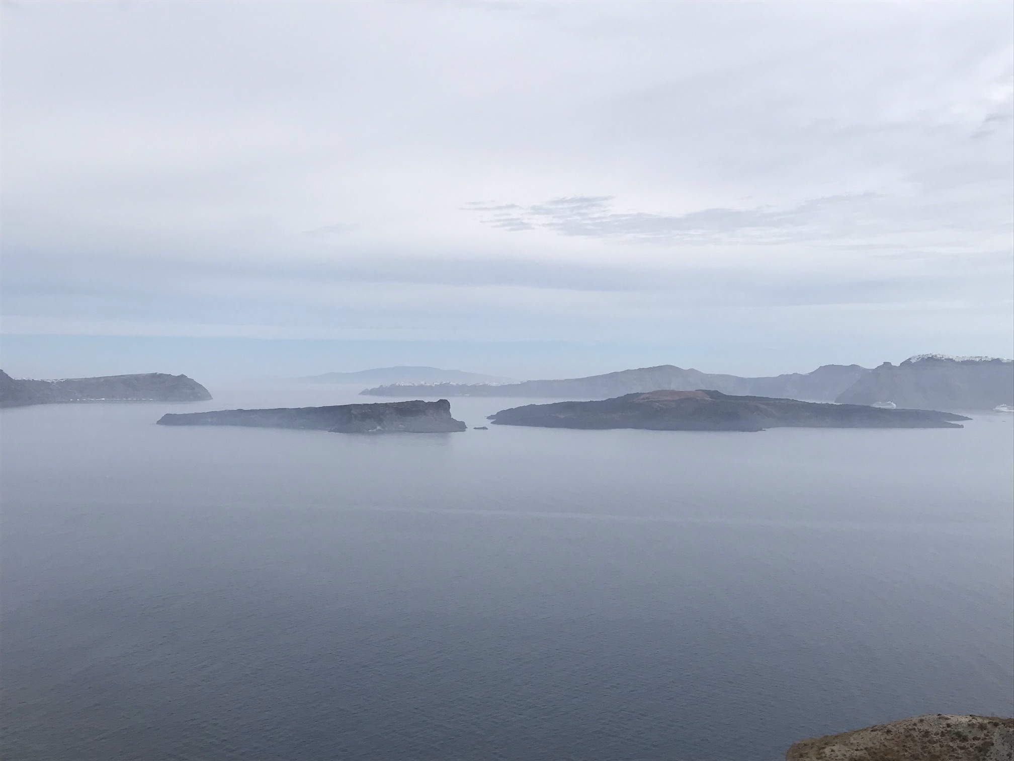
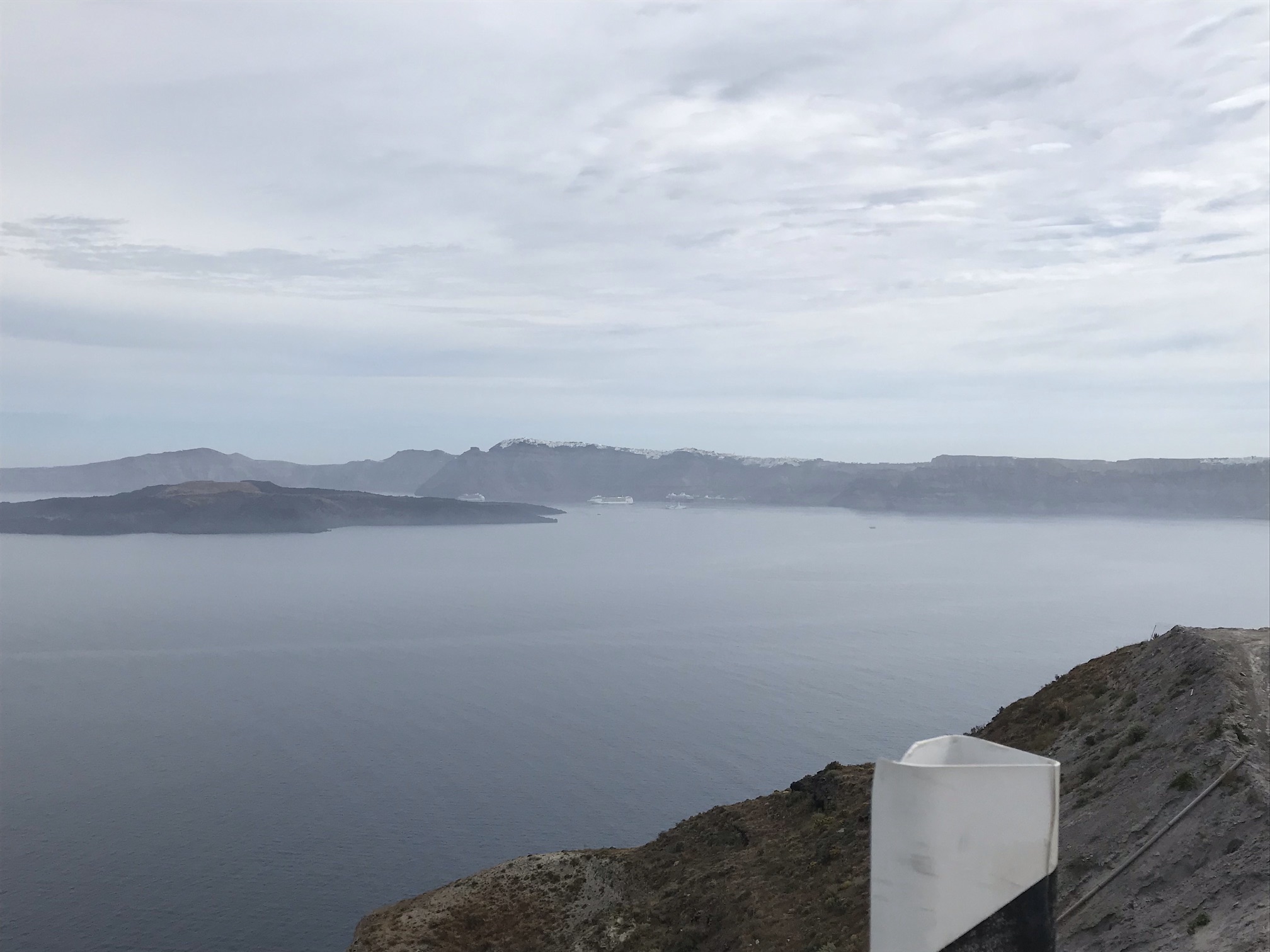
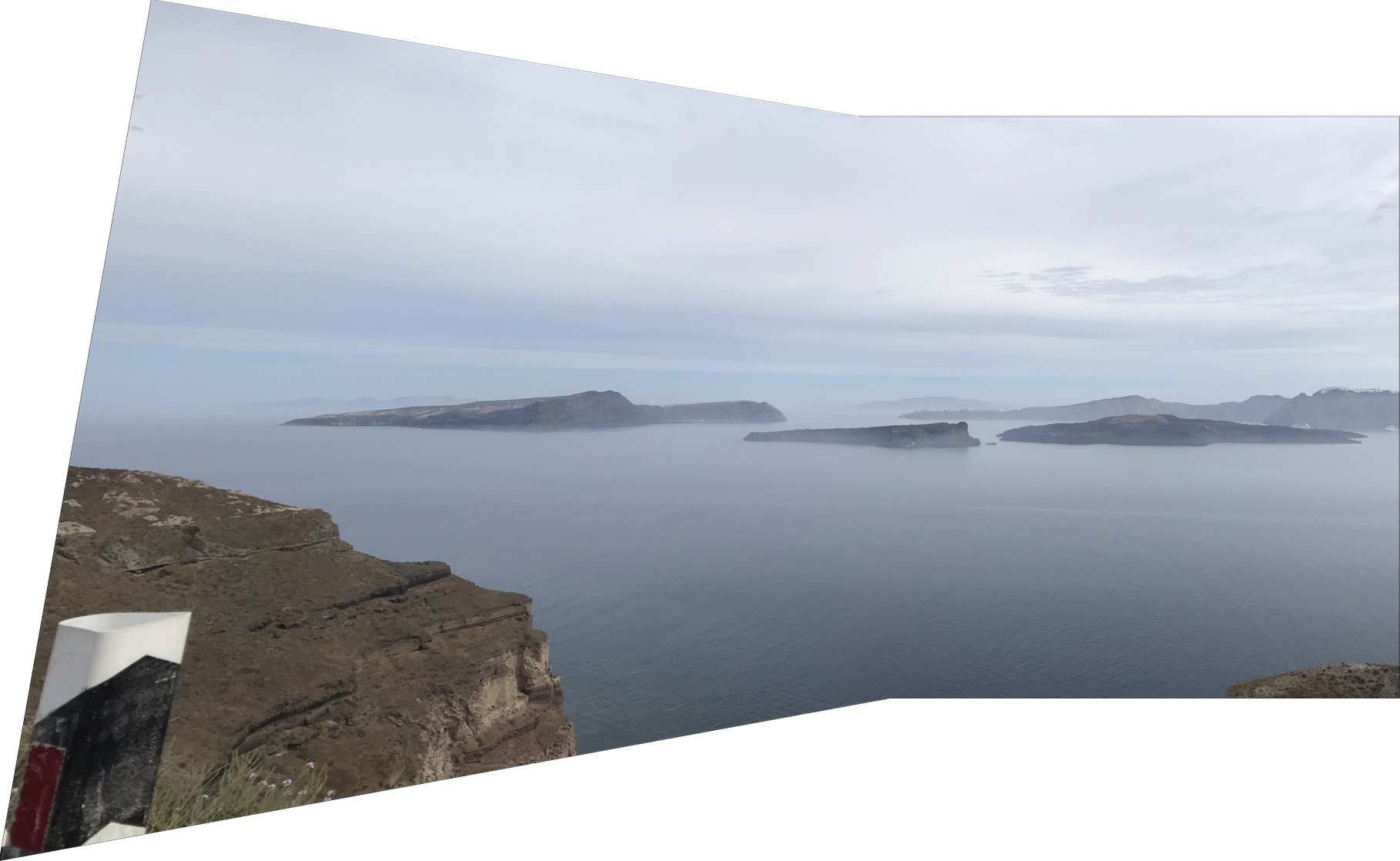
| Manual Mosaic - Island (First 2 images only) |
|
| Autostitched Mosaic - Island |
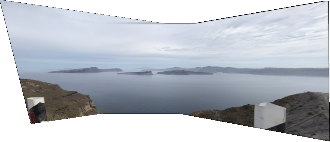 |
I enjoyed reading through the paper and implementing each section. ANMS was particularily interesting, and from my experiences with working through the project, it appears to be the slowest part of the autostitching algorithm. This is part of the reason why I had to downsample the original images or increase the min_distance parameter when getting Harris corners. RANSAC is also a very simple and neat algorithm for reducing outliers that I enjoyed learning about and implementing.