This is some basic, sample markdown.
I started with the equation Hp = p' to see how to create the matrix A and solve for Ax =b. I noticed that I could rewrite Hp = p' as 3 separate linear equations.
ax + by + c= x'
dx + ey + f = y'
gx + hy + 1 = 1
Using this idea I made each row of the matrix A an equation by giving it 8 columns. For the first row, the corresponding b element was x', and the row in A was x, y, 1 followed by 0s. The second row was three zeros followed by x, y, 1 followed by zeros with corresponding y'. The last row follows the same pattern. By doing this for each point, I solved the least squares equation of Ax = b to get the homography and converted it back to a matrix.
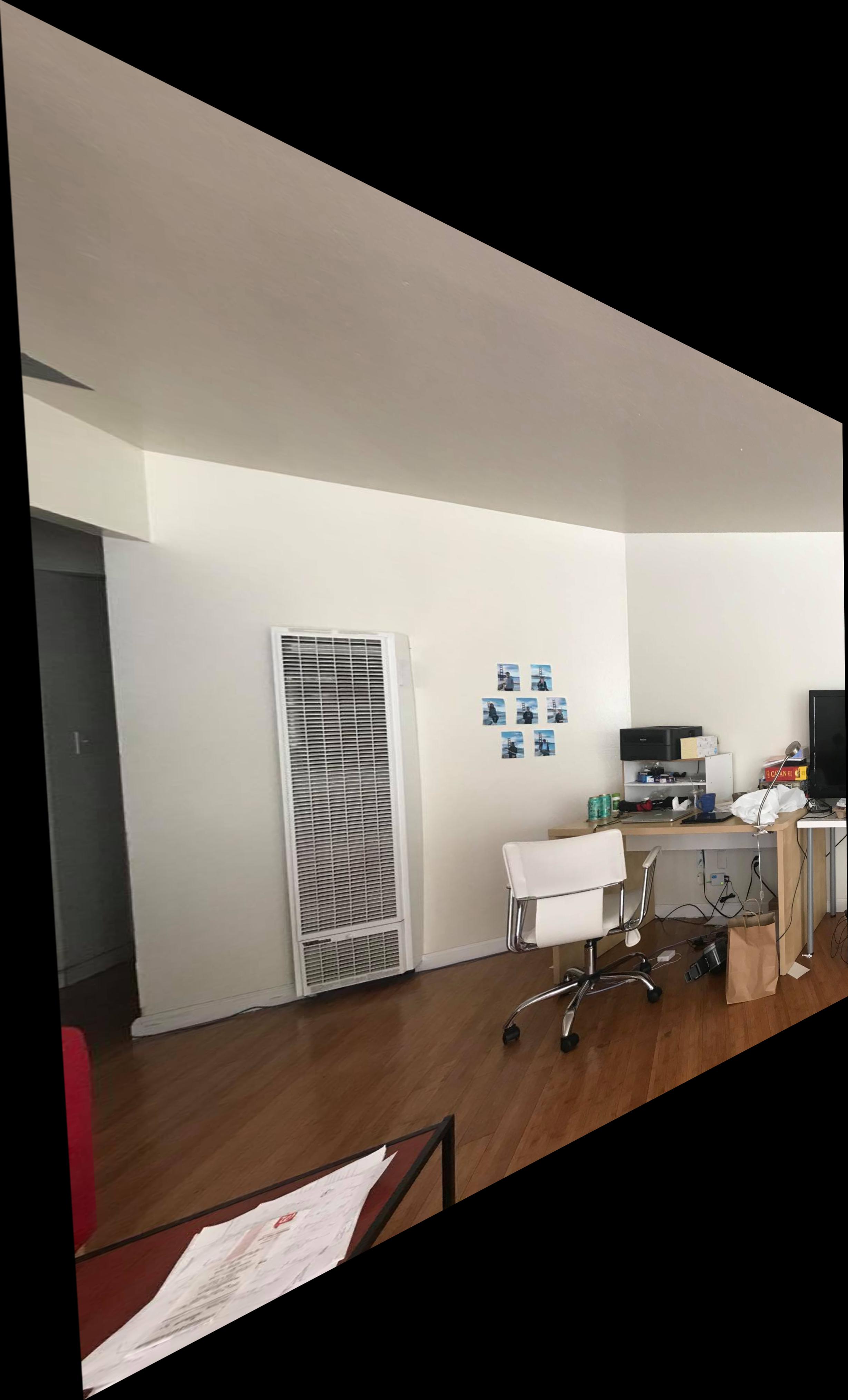
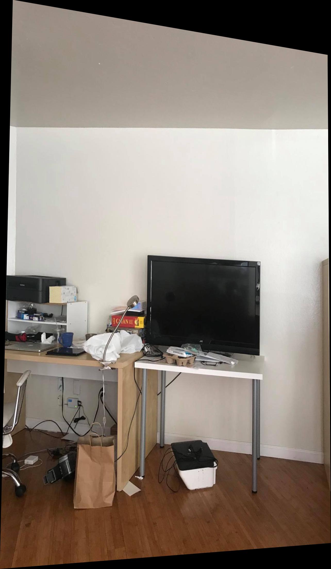
After obtaining the homography based on predefined points, we can begin image warping. The way that I approached this was to use inverse warping. I first computed a bounding box for the transformed image. Then, I created a matrix of each pixel of the bounding box and multiplied it by the inverse of the transformation. For each of these points, I used cv2's remap to get the linearly interpolated pixel value from the image.
For rectification, I simply picked 4 points that I approximated to be rectangular, and guessed another 4 points to be a rectangle on the new image. I computed the homography and then applied the warp.
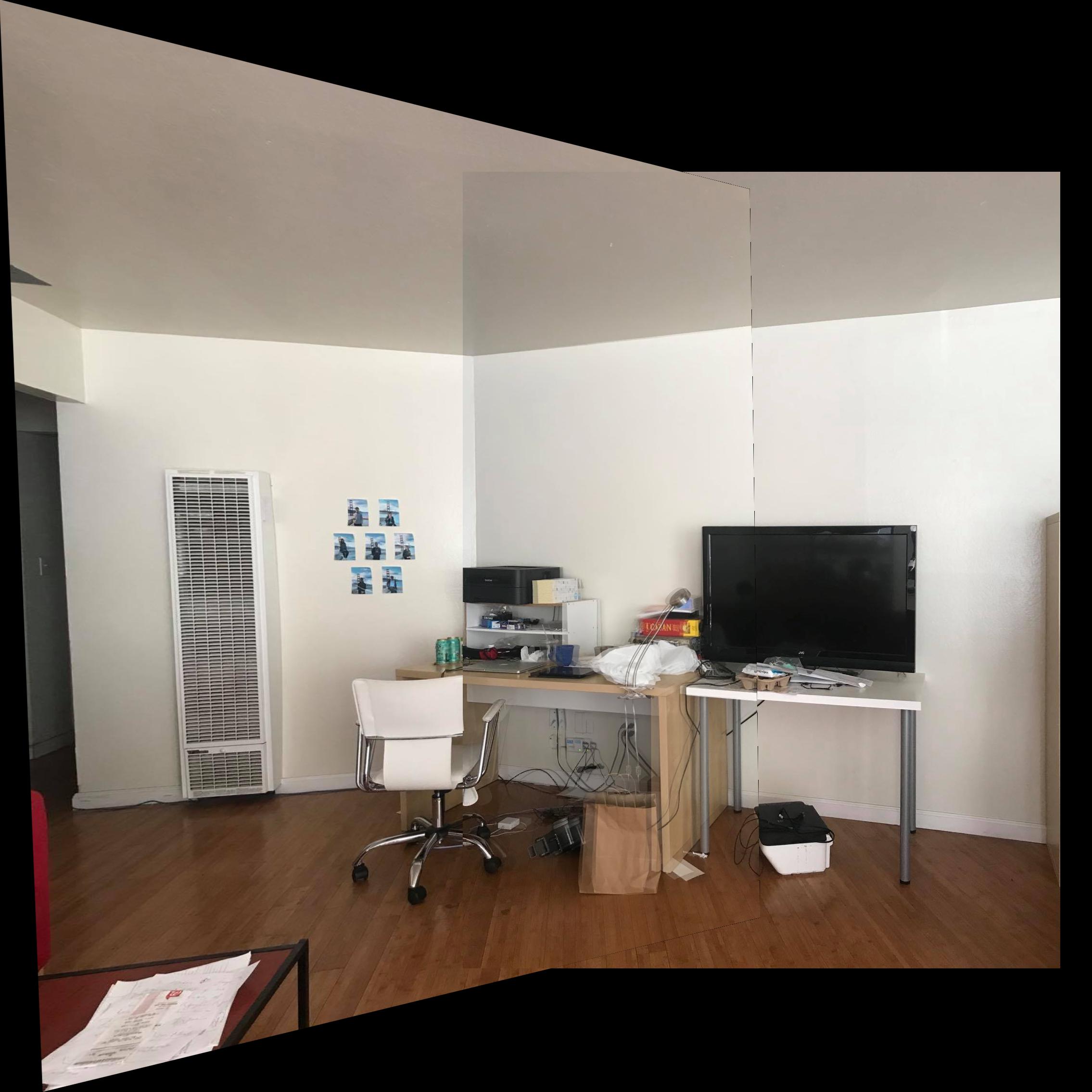
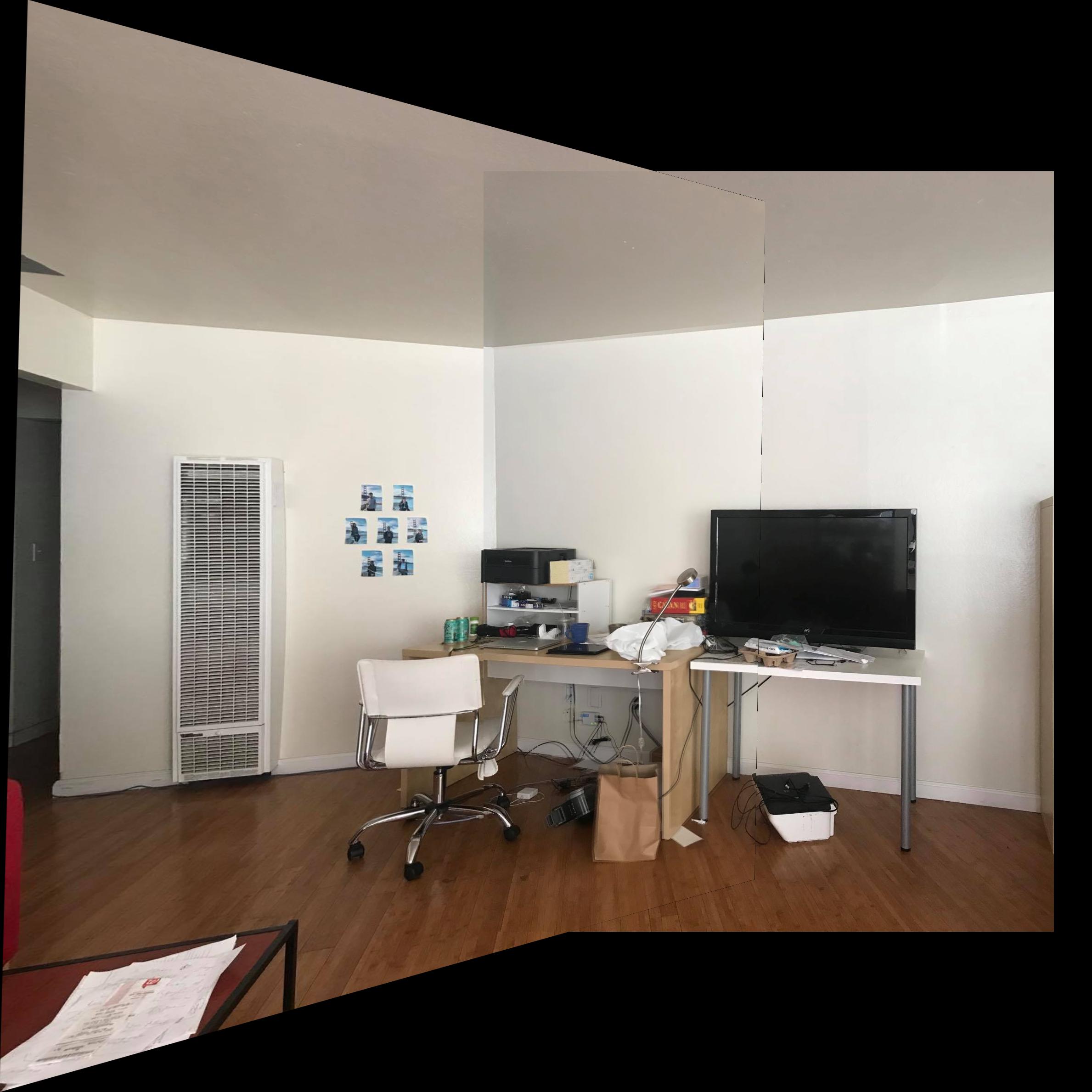
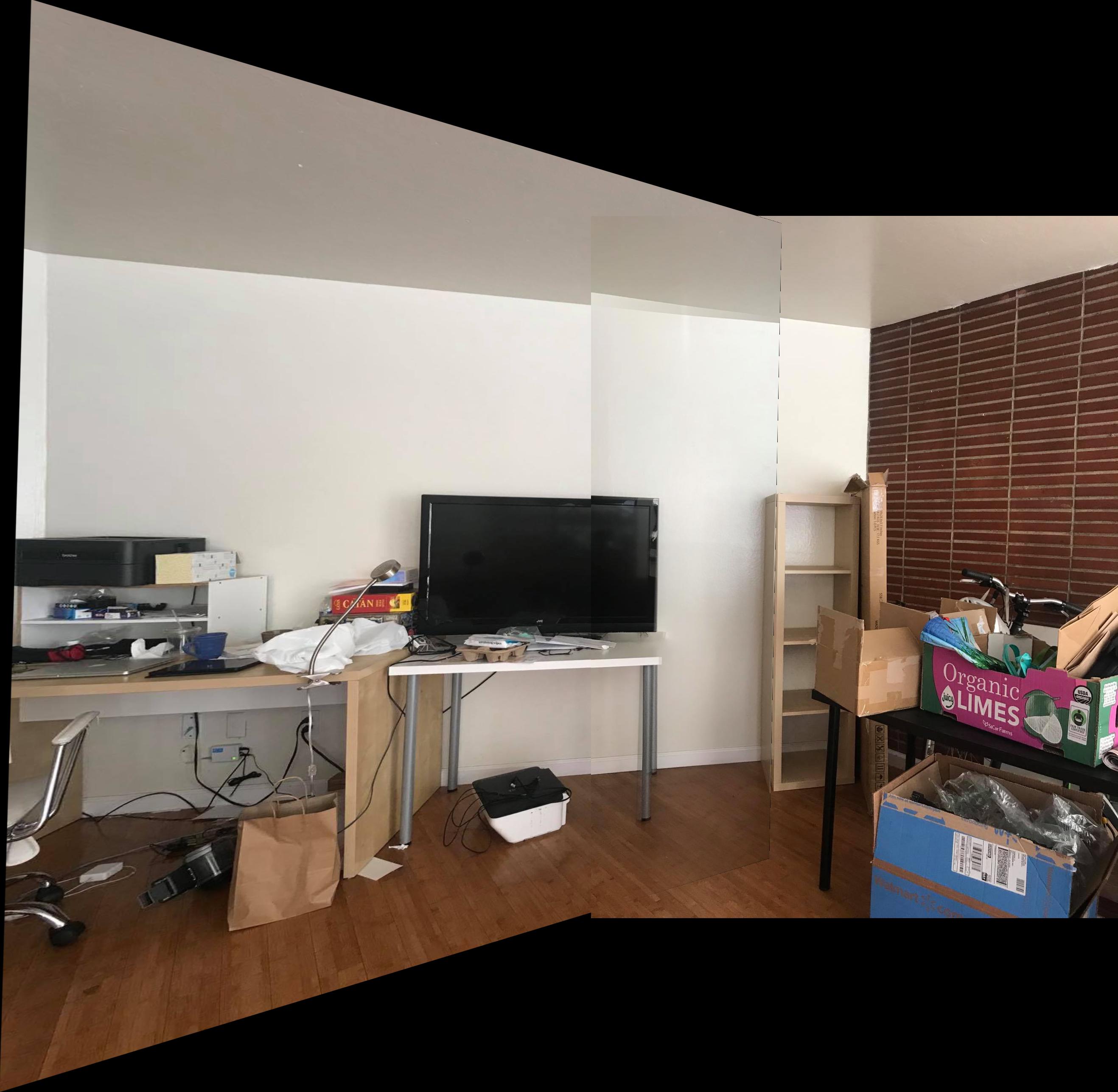
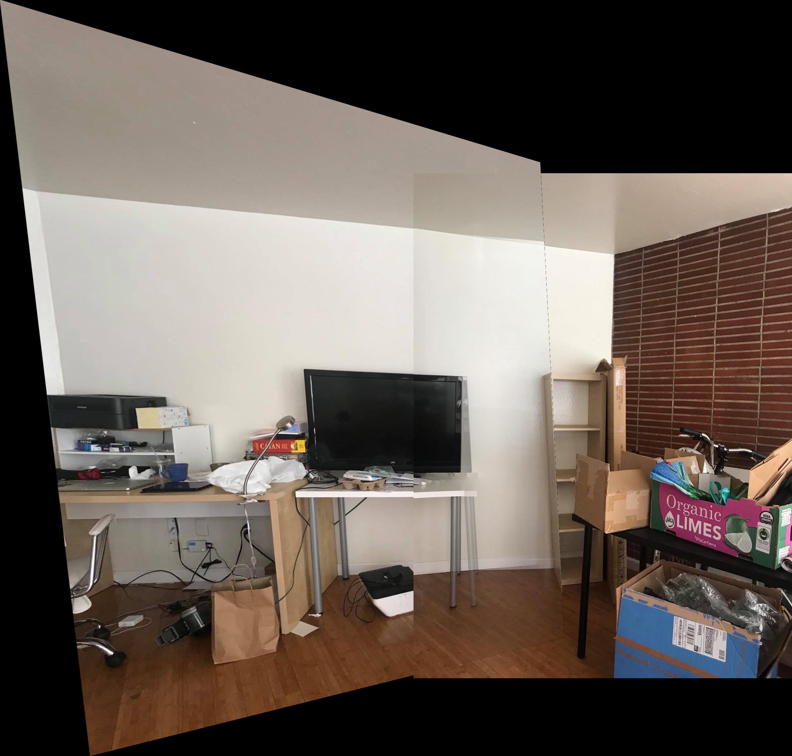
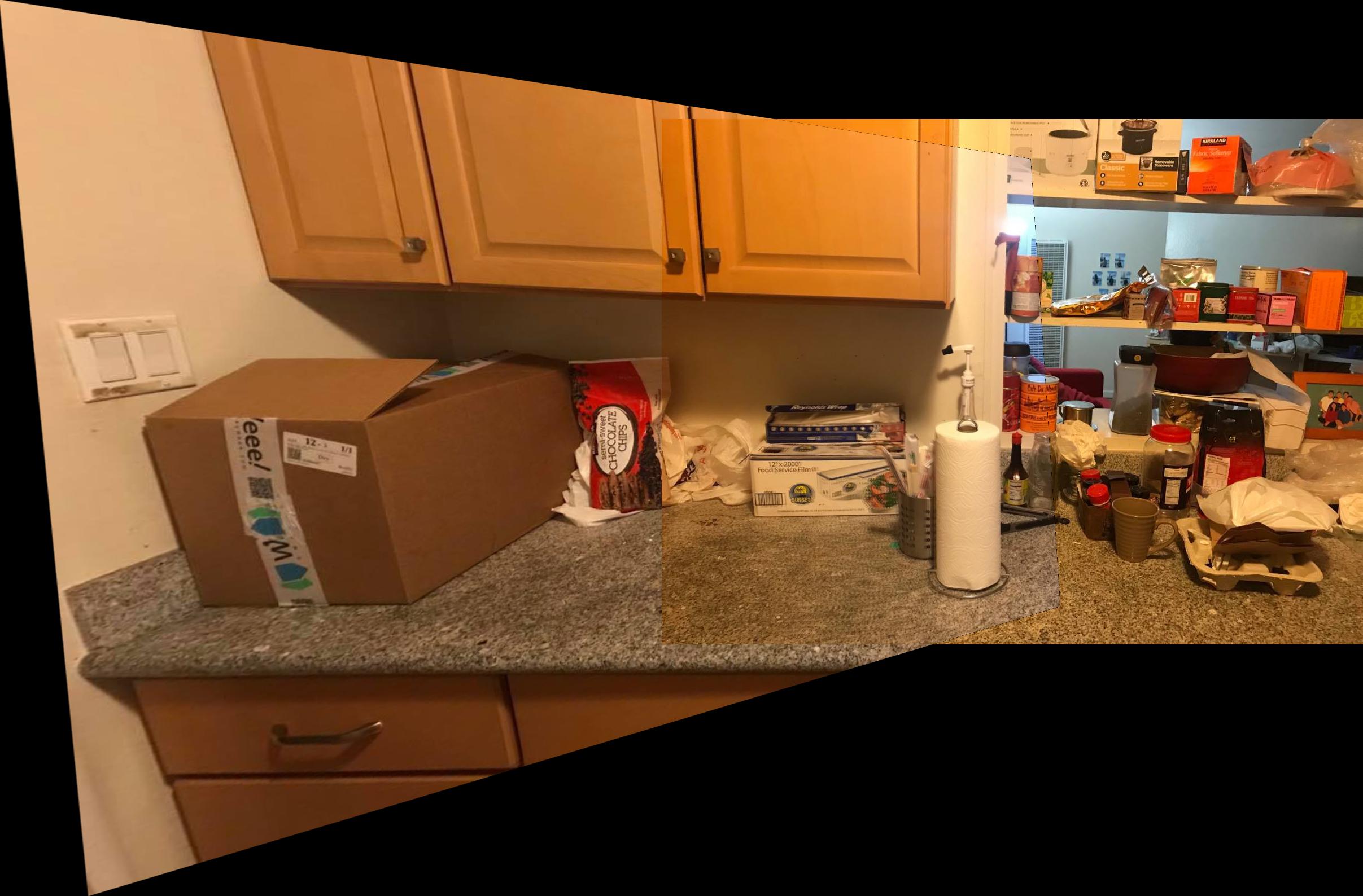
Blending was done by first creating 4 canvas images. The first one contains the warped image. The second one contains the second image. The third canvas is a mask for where the images overlap. The last canvas is a gradient to vary the alpha over the mask. After creating the canvases, a linear combination is taken in order to create the blended image.
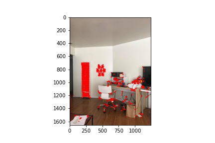
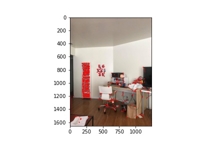
Interest points are first selected using multi scale Harris corners.
For each interest points, we get the harris value of the point. Then, for every other interest point, if the harris value is less than 0.9* the original point's harris value, we calculate the squared distance between the points and add it to a list. We then calculate the minimum suppression radius (squared distance) for that point. This restricts the number of interest points and ensures a better spacial distribution for the interest points.
Feature vectors are created from each interest point by first sampling a 40x40 block around the interest point. A gaussian blur is applied and the block is down sampled into an 8x8 block. Then, we convert this into a 64 length vector.
We want to find matching features between two images. To do this, we look at the error for each pair of features in each image. If the ratio of the nearest neighbor and the second nearest neighbor is less than a certain threshold, we consider those features a match. At the end, we return a list of matching features..
Finally, we need to compute a Homography between the matching features by using the RANSAC algorithm. For a set number of iterations, we pick a random sample of 4 matching features. We then compute a Homography between those matching features. Now, we can find all inliers for all matching features with that homography by calculating the SSE of predicted vs. actual points. If the error is less than a certain threshold, we append the feature's corresponding interest point. Lastly, we want the Homography that produces the greatest number of inliers in all of our iterations. At the end, for this maximum set of inliers, we compute a Homography based on these poionts.
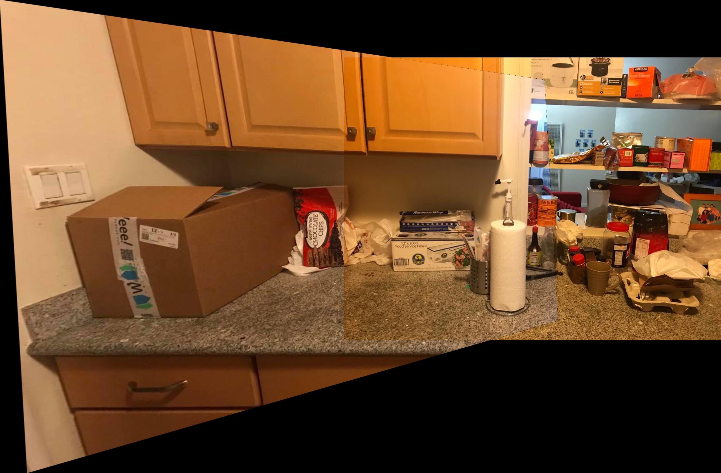
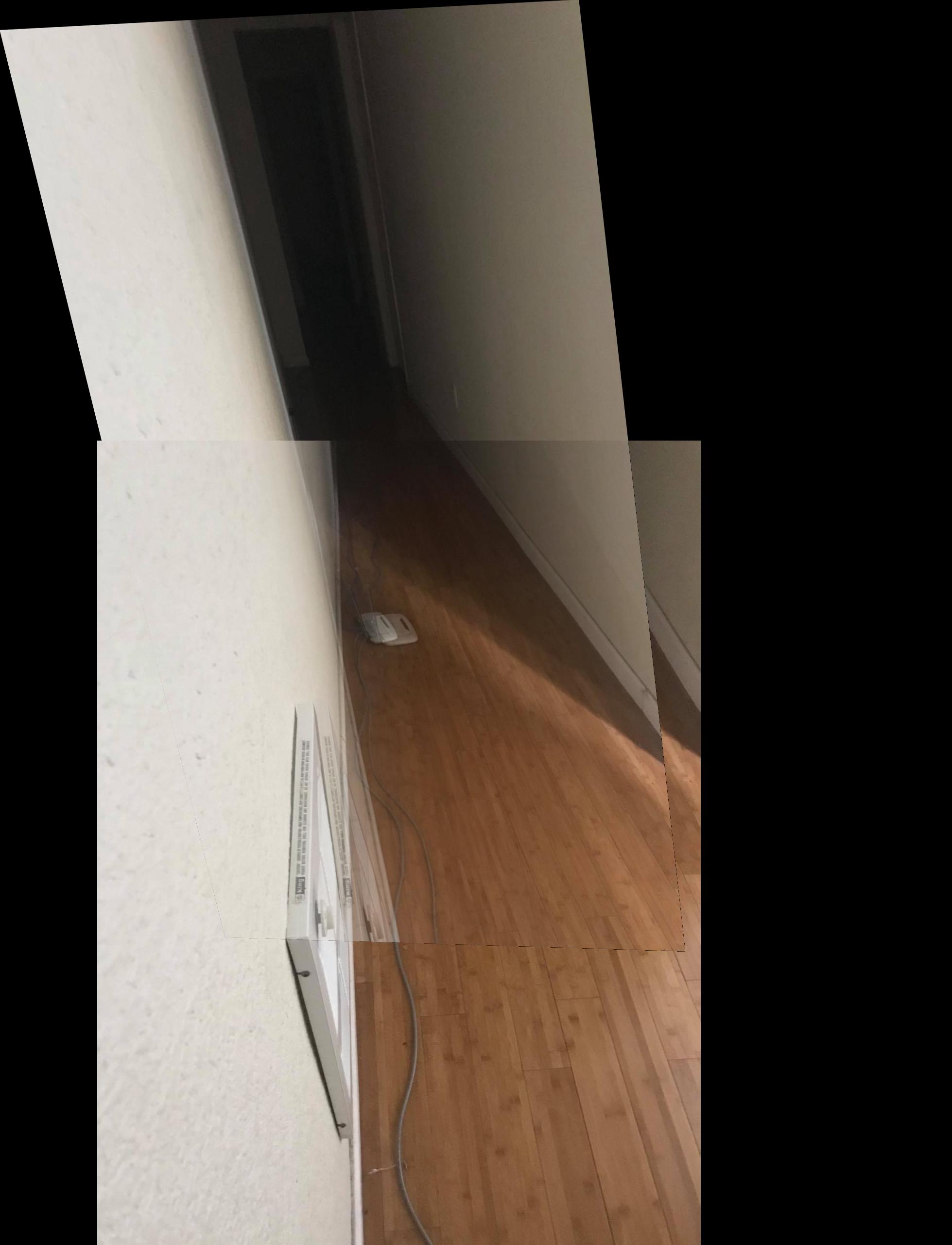
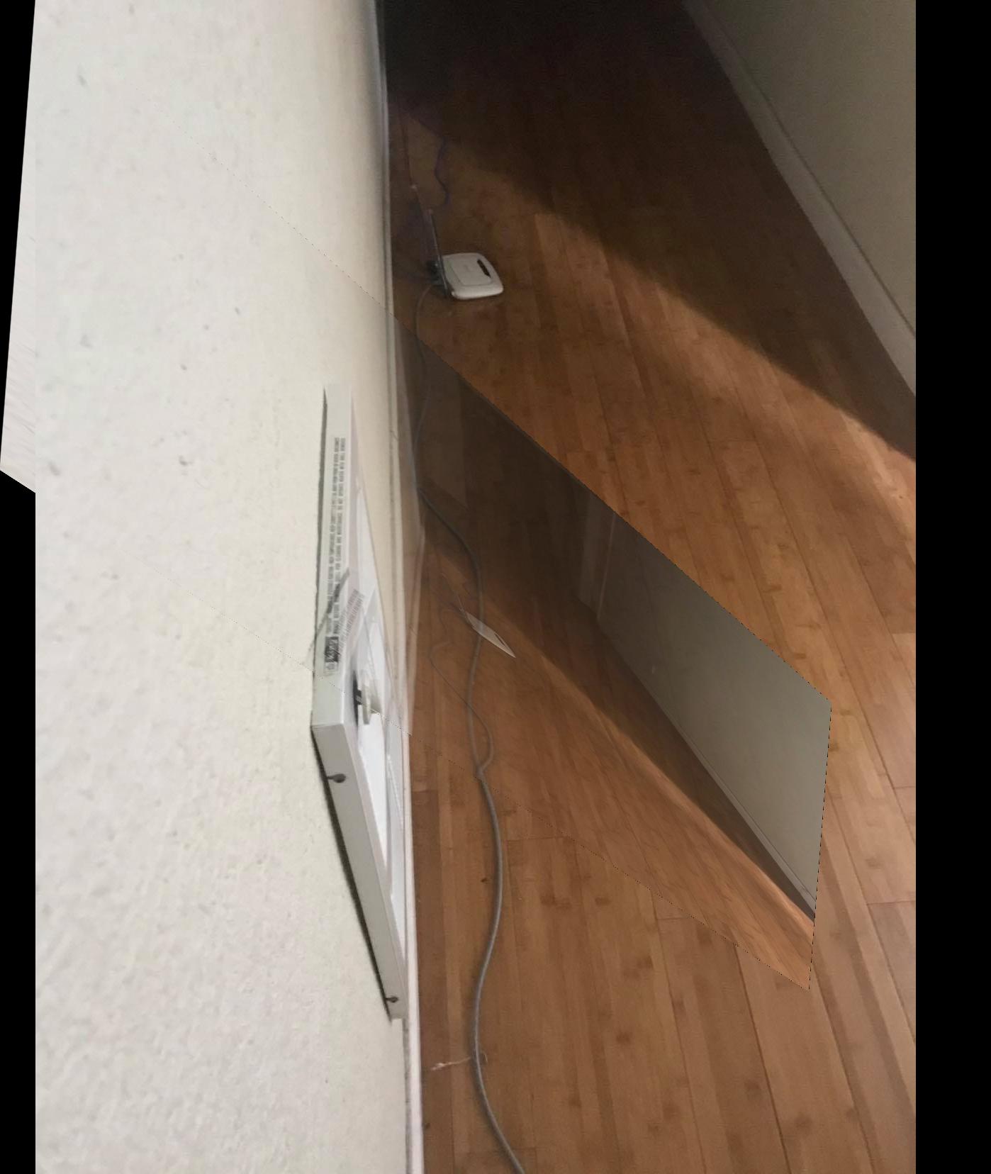
In the first part, the coolest thing I learned was homographies and Image Rectification. I didn't really think that a simple 3x3 transformation matrix could completely transform an image to look like it was taken from a different perspective. In the second part, I thought feature detection and matching was really cool. I was surprised at how well the algorithm worked. One thing that could've been improved was the blending algorithm. To start, there are some noticeable artifacts depending on how aligned the correspondance points are. I had hoped to reduce this by applying a gradient to vary the alpha when blending, but this wasn't enough. The blending function also had issues when blending certain images due to some bounding issues. It also only blend a warped left image to a right image. I initially wanted to have functionality for multiple image mosaics, but due to lack of time I was unable to implement it.