Photo Mosaics & (Auto) Stitching

Part A: Image Warping and Mosaicing

1. Shoot the Pictures

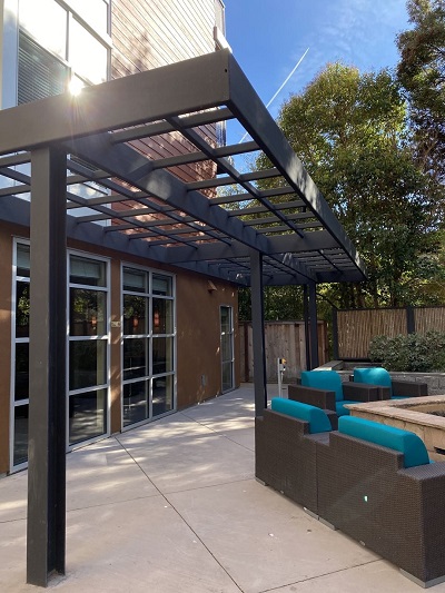
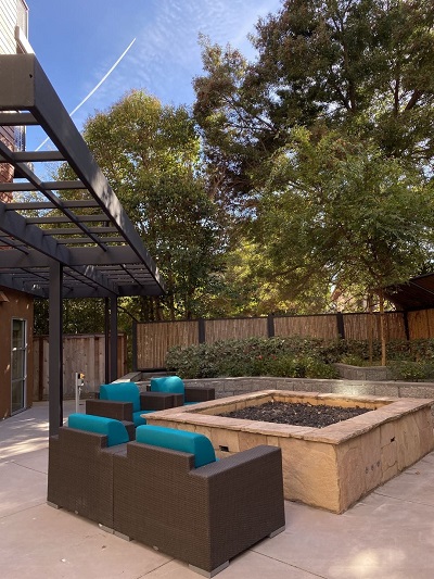
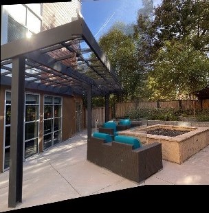
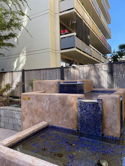
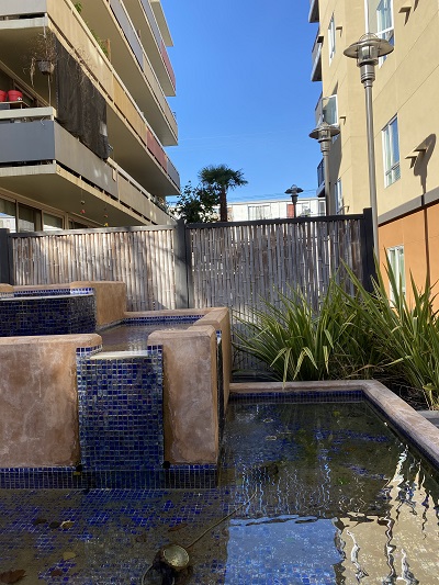
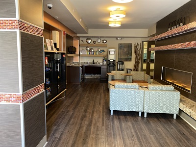
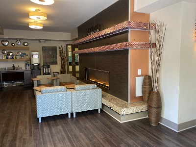
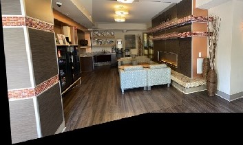
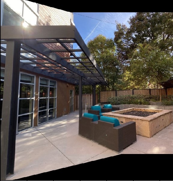
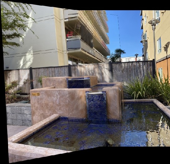
I took these three images in my apartment's courtyard. In order to make mosaicing easier, I overlapped 50% of the images. I also made sure to rotate the angle without changing the position of shooting point.

2. Recover Homographies

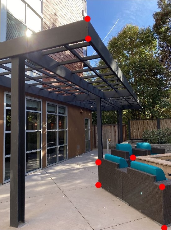
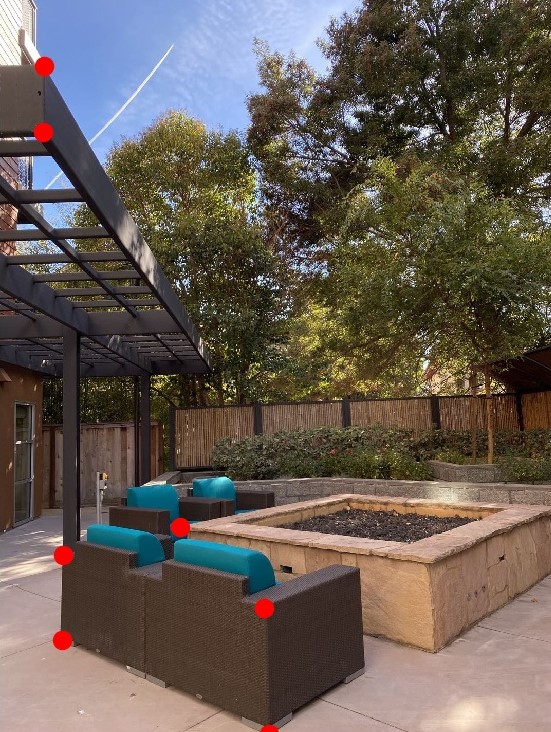
Since the two pictures are in different perspective, the first thing I need to do is project one into another's perspective. I first calculated a homography matrix H by solving a system of linear equations. Since the degree of freedom for H is 8, we only need 4 data points to calcualte it. To make the result more accurate, I chose 7 points depicted below to calcualte the projective transformation. Since there are noise in the data, I used least square equation to calculate H.

3. Image Rectification/Warp the Images

After calculating a homography matrix H, I am ready to warp the image. I used inverse warping which takes the following steps: For each pixel point in the destination image, I applied H_inverse to find the corresponding pixel value in the original image.

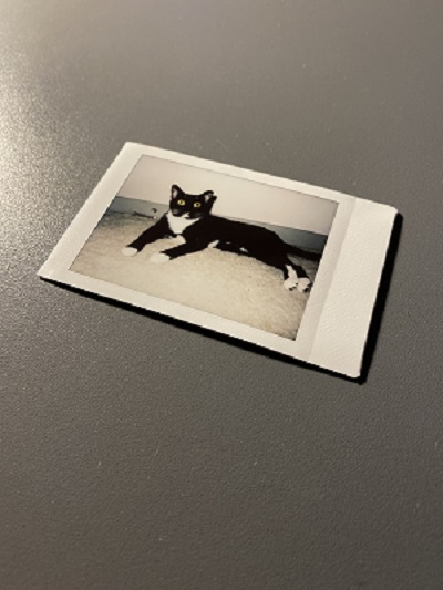
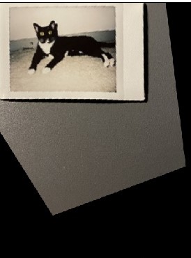
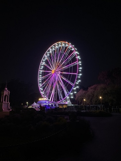
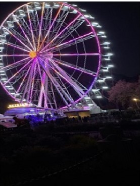
Warping can also be used to rectify images. Here I show a few example of pictures taken at an angle, and warp them back to front-view:

3. Blend Images into Mosaic

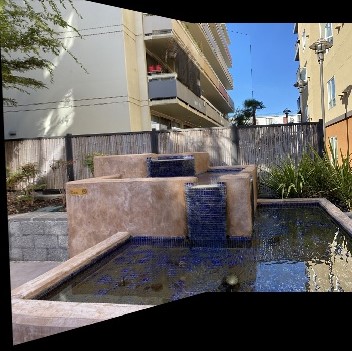
Finally, we're ready to blend images into mosaics. I used a linear blending where I created a mask to add 50% each of the overlapping part of two images into the result, then add the non-overlapping parts. The black parts are due to image projection. The image pairs and resulting mosaics are shown below. I took these pictures from my apartment building.

Courtyard View
Fountain View
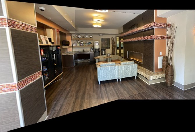
Lounge View

5. Learnings from Part A

Part A was very fun to work on, as we get to take pictures ourselves and be creative with it. I learned a lot through calculating homography and warp the images together. Even though it's very time consuming to stitch the images perfectly, I still enjoyed it a lot.

Part B: Feature Matching for Autostitching

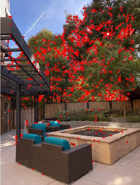
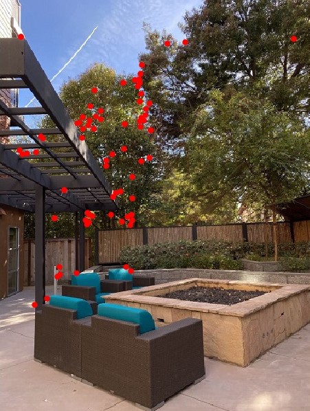
1. Detect Corner Features

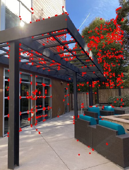
Part B improved from Part A in which we no longer need to find same features in two images manually. Instead, we will automatically detect them using techniques in: “Multi-Image Matching using Multi-Scale Oriented Patches” by Brown et al. First of all, we use Harris Corner Detection Algorithm to automatically find all the corners in eacn image. The result of detection is shown below:

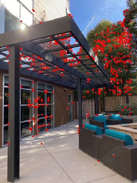
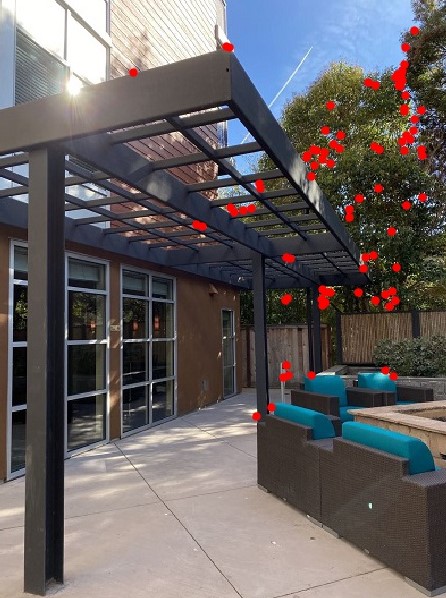
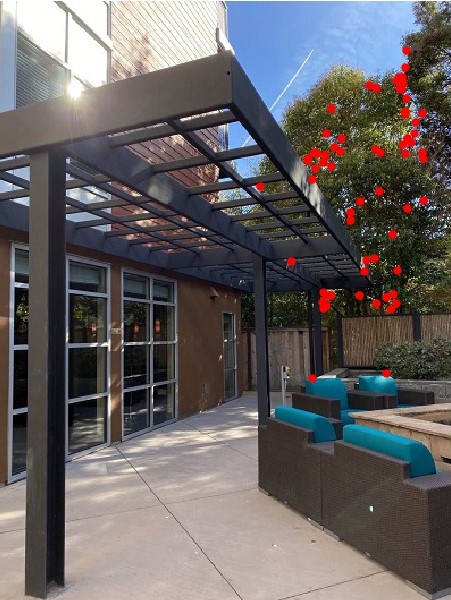
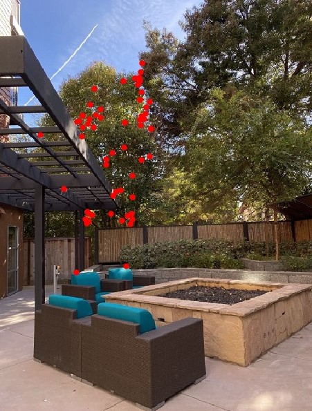
2. Adaptive Non-Maximal Suppression

Although Harris Corner Detection gave us large amount of corner points, we want to filter them and make them spread out through the entire image. Therefore, we use Adaptive Non-Maximal Suppression, which is described in the equation below, to filter our points.

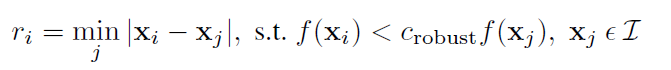
We first calculate the min_suppression_radius for each corner point, then we chose 500 points that have the maximum min_suppression_radius as our interest points. The result after filtering is below:

3. Feature Descriptor Extraction & Matching

After we have all the corner points, we create feature descriptors for each point so that points with similar feature could be matched. Our features are 8x8 squares extracted from 40x40 pixels points around the corner points. We then applied a Gaussian filter to blur it. Here are some examples of our feature descriptors from two images:

We then performed feature matching: For each feature in image1, we found its nearest-neighbor (1-NN) in image2 by calculating the distance between the two feature descriptors. Then, we need to eliminate bad matchings. For each pair of matchings, we keep it if the fraction between distance to its nearest neighbor and distance to its second nearest neighbot is smaller than some threshold. That is, error(1-NN) / error(2-NN) < threshold. We set threshold=0.4 according to the paper. In this way, we successfully matched corner pairs, and the result is shown below.

4. RANSAC

Even after feature matching, there could still be many outliers, as least-square is vulnerable to outliers. Here, we used a method called RANSAC to filter out outliers. The procedure is as follows. In each iteration, we:

1. Select four random pairs of points
2. Compute the homography matrix H.
3. Compute inliers where SSD(p’, H(p))) < epsilon

I set epsilon=1 after some experimentation.After 100 iterations, we keep the largest set of inliers found to be our final matching points. The final matching points are shown belos:

5. Blending Images

Finally, after all the automatic feature detection, we are ready to blend our images! The blending procedure is the same as Part A, where I calculate homography matrix H based on the set of matching points, and warp one image into another's perspective. Here I compared mosaics using manual feature detection and automatic feature detection, and we can see that automatic detection is a lot better. Some examples are shown below:

5. Learnings from Part B

I think this is a very meaningful project as I have learned a lot through reading paper and replicate its results. It furthered my understanding to image processing concepts, and allowed me to explore creatively on my own. Overall I have enjoyed this project a lot.