Part A: Image warping and Mosaicing

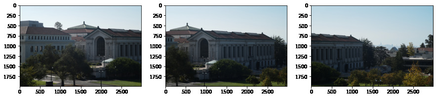
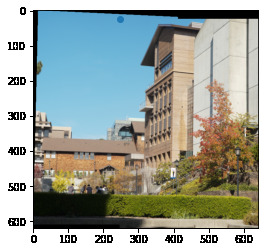
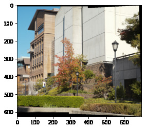
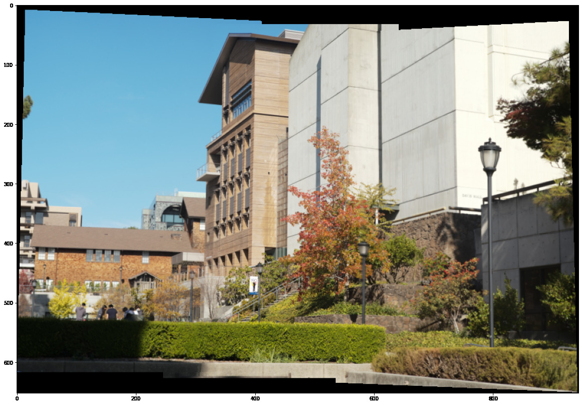
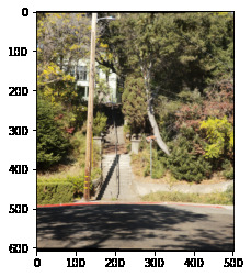
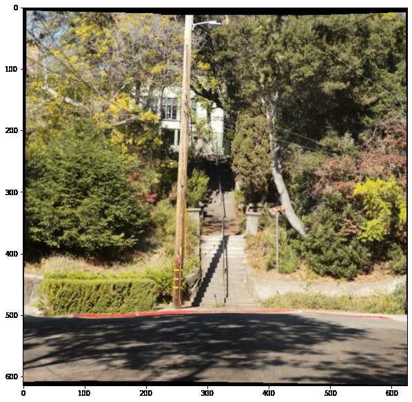
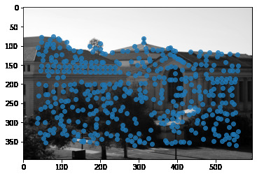
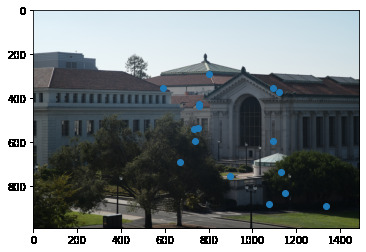
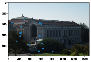
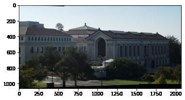
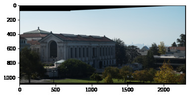
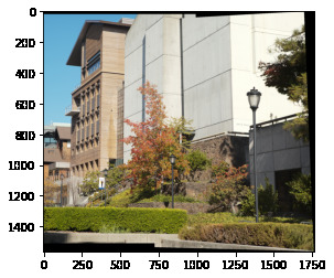
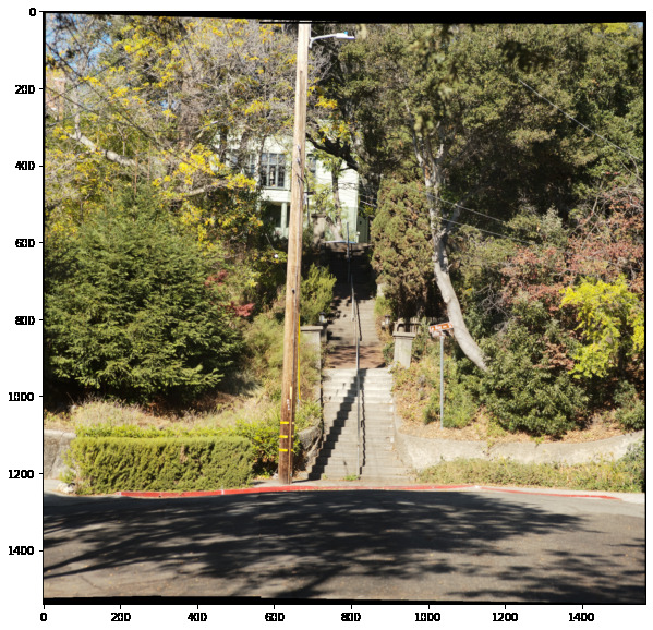
We're going to be doing some mosaicing! This is when multiple images from the same point are combined into one large one using homographies. To capture images I used a digital camera with a 90mm lense. All images for a specific mosaic were taken at the same exposure to keep the color consistent. Here's a sample of some of the pictures I took of doe library

1. Computing homographies

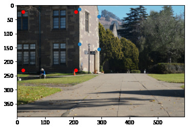
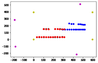
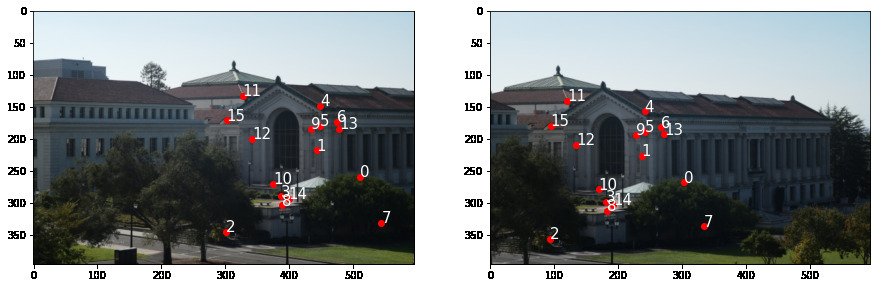
In order to compute homographies, we need to determine points in the intersection of two images where they correspond. This transformation should warp a given part of an image on top of the corresponding part of the other. We first start by choosing correspondence points.

Little Bell/Whistle 1: We also fine-tune our point selections by taking a small 160x160 pixel section around each corresponding pair of points and correlate the two patches after normalization. This lets us determine the error in our alignment and we can select the point of maximal correlation to set the two points to.

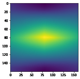
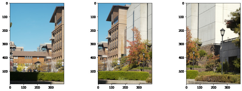
After finetuning, here are the points correspondence we get on each of the images.

Now we can make our homography!

If we want to map the point a = (x, y, 1) to another point b = (u, v, 1) We can write out Ha = b as a system of 9 equations, we get, for each point given, the 2x9 matrix

[[-x, -y, -1,  0,  0,  0,  u*x,    u*y,  u],
 [0,   0,  0, -x, -y, -1,   v*x,    v*y , v]]

If we write the 3x3 matrix H as a vector h=[h11, h12, h13, h21, h22, h23, h31, h32, h33], we can solve the system Ah=0 Where A is what we get if we stack each of the above matrices for each point. We can then find the best non-trivial solution by computing the SVD of A=USV' and taking h as the last vector of V, then normalizing it such that h33=1.

Little Bell/Whistle 2: It turns out solving the above system can be somewhat numerically unstable, and this can lead to slight errors in the alignment of pixels. I explored a variety of other potential solutions.

One method of doing so is to "condition" the input points such that they converge to a better solution. As explained here, we can compute a new transformation, T which transforms the points such that their mean is at the origin and their average distance from the origin is sqrt(2) (this is done by scaling by the sample standard deviation of the points). We then output T^-1 HT so that our transformation "conditions" the points, applies the homography, then reverses the conditioning.

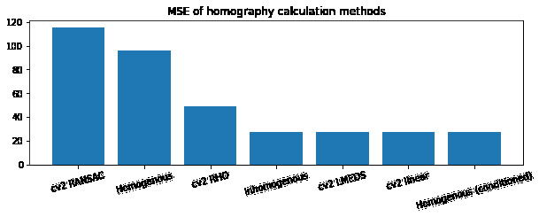
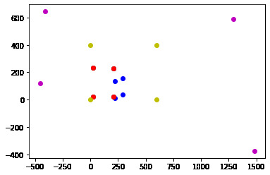
Let's look at the error we encounter when solving the normal homogenous system. Below is the difference between the transformed points and the desired output:

    [[  0   0   0   0  -6 -14 -20  -1 -20  -5   5   0 -11 -11 -12  -2]
     [  0   0   0   0   5   2 -13   9  15  18  16  -4  -2  -6 -22   6]]
    MSE 97.90625

This difference is as much as 20 pixels! When we apply our conditioning method, we get a much closer result:

   [[ 14   3  -2   3   3   2  -7   3  -1  -2  -2   1  -4  -5  -6   2]
    [  7   1   1  -4   4   5  -5   3  -1   1   3  -3   2  -2 -18   4]
    [  0   0   0   0   0   0   0   0   0   0   0   0   0   0   0   0]]
    MSE 27.8125 

Wow! Our Mean Squared Error (MSE) dropped from ~98 to ~28! Sweet!

Another potential way of solving this system which doesn't rely on computing the svd is to set h33=1 to begin with and then solve for Ha=b with 8 unknowns. This yields a very similar system as listed above and instead we can solve Ah=B where A is our system and B is all the b points flattened.

This also seems to converge to a similar solution as our conditioned SVD method did! Fascinating!

    [[ 14   2  -2   2   3   2  -6   2  -1  -2  -1   1  -4  -6  -6   2]
     [  7   1   1  -4   4   5  -4   4  -1   2   4  -4   2  -2 -18   4]
     [  0   0   0   0   0   0   0   0   0   0   0   0   0   0   0   0]]
    MSE 27.65625

I then became super curious as to how good different methods were at computing these homographies. I tested all of my code against implementations in OpenCV (RANSAC, RHO, LMEDS, and linear) to see how they performed on our system. Unsurprisingly they all converged to a very good solution somewhere around the conditioned homogenous system. These other algorithms like RANSAC are also able to detect outliers however, so for less-cleanly defined points, they may converge to higher MSE-yielding solutions which are in fact better than our simple linear least squares approximation.

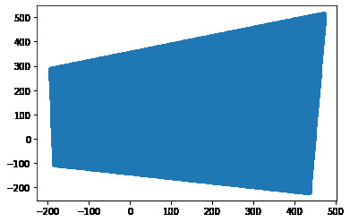
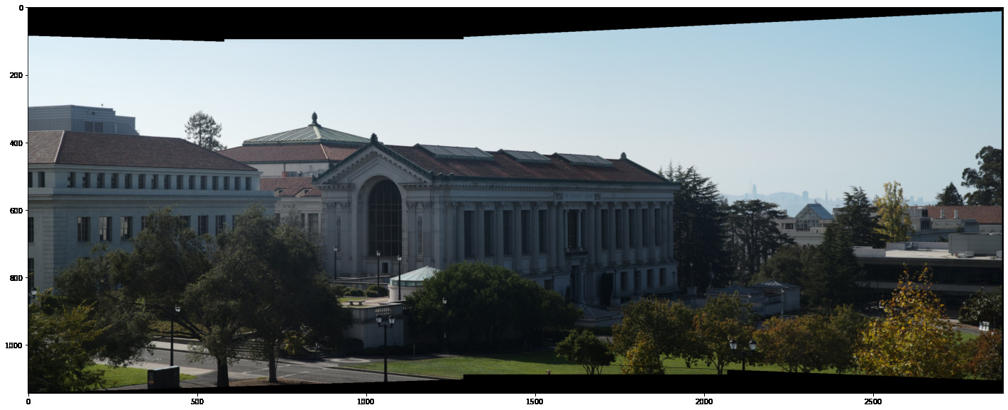
We can now apply the computed homographies to our images!

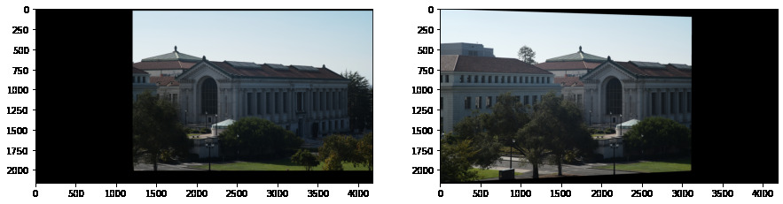
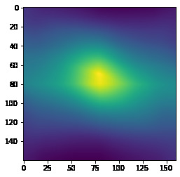
By detecting where the images' bounding boxes intersect we can create a nice smooth gradient between them and use a combination of masks to blend them together.

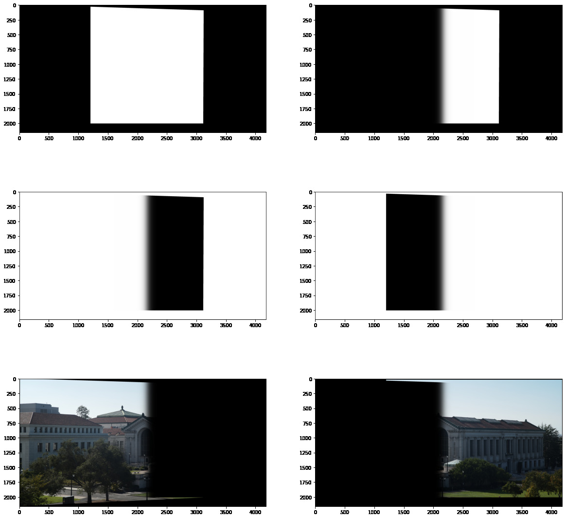
Doing this for the other pair of images we get:

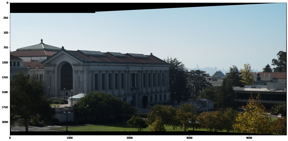
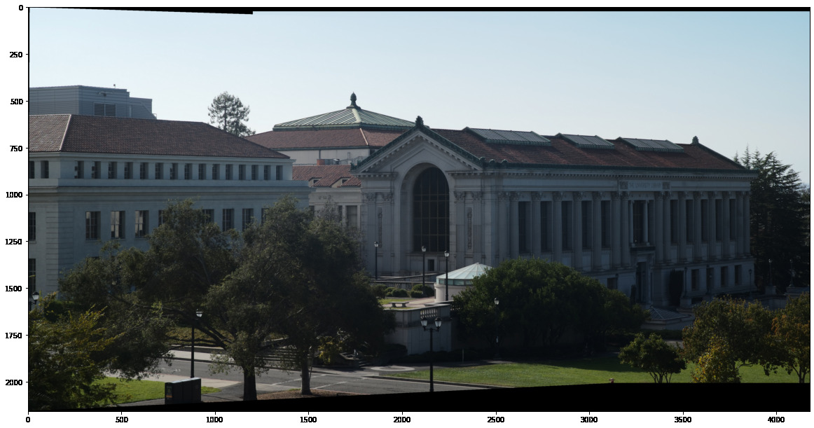
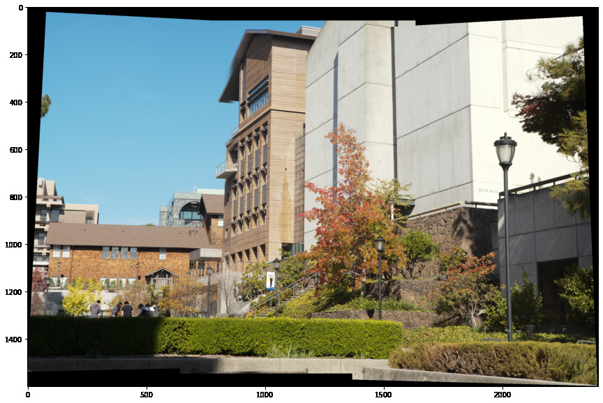
With some tricky index math we can then combine these two blended images together into one sweet mosaic:

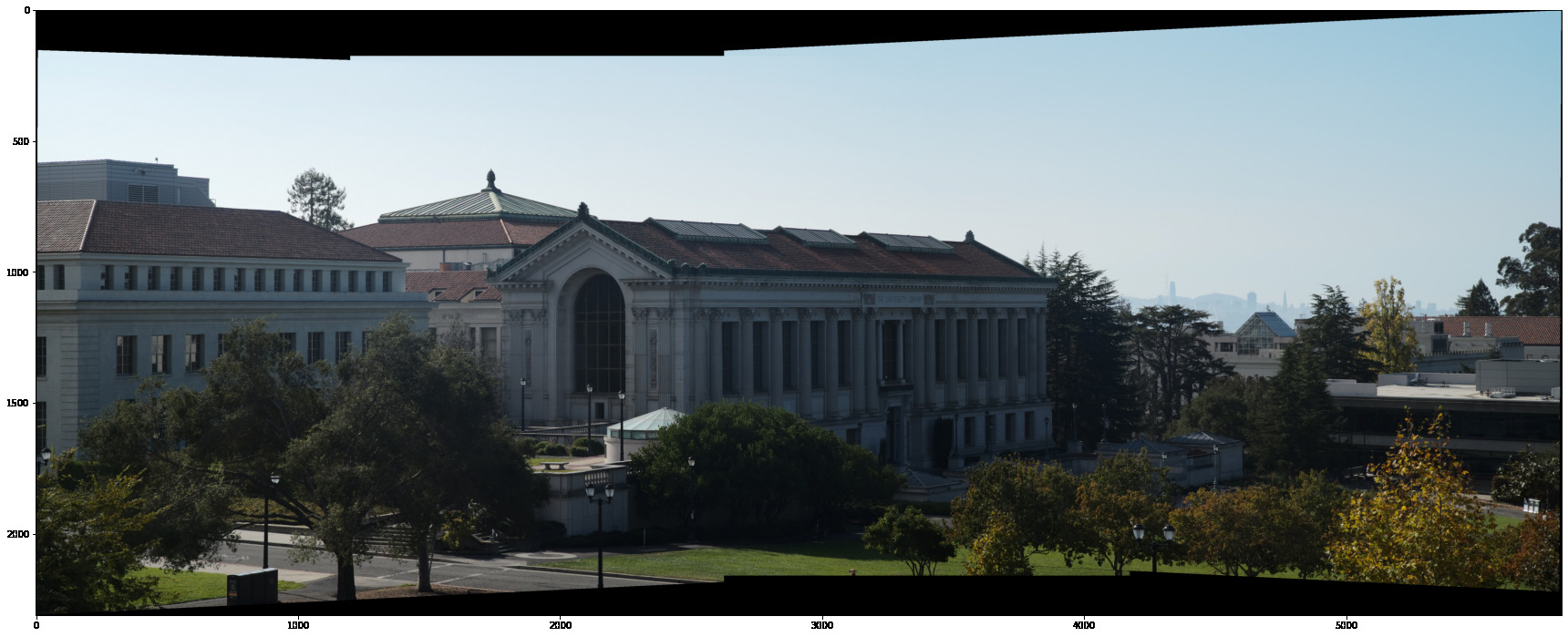
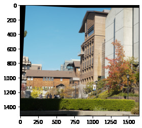
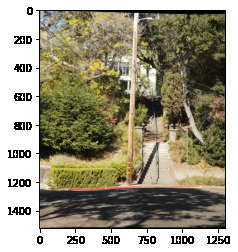
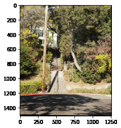
Here's how it performed on a couple other images I took:

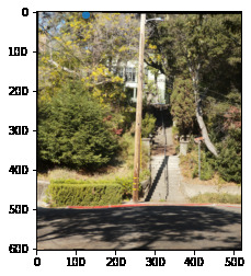
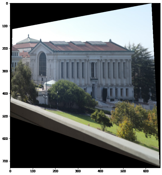
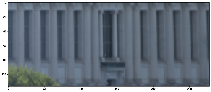
Rectification

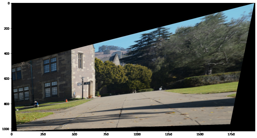
Another thing we can do is transform our images such that surfaces which were some non-rectangular box in our image before now become rectangular in the eyes of our camera:

The coolest thing I learned in this first part was definitely the different methods of finding homographies. It's funny to think that certain systems can be changed to make them more easily solvable, even when there is a unique global minimum we want to reach.

Part B: Automated Homography Computation

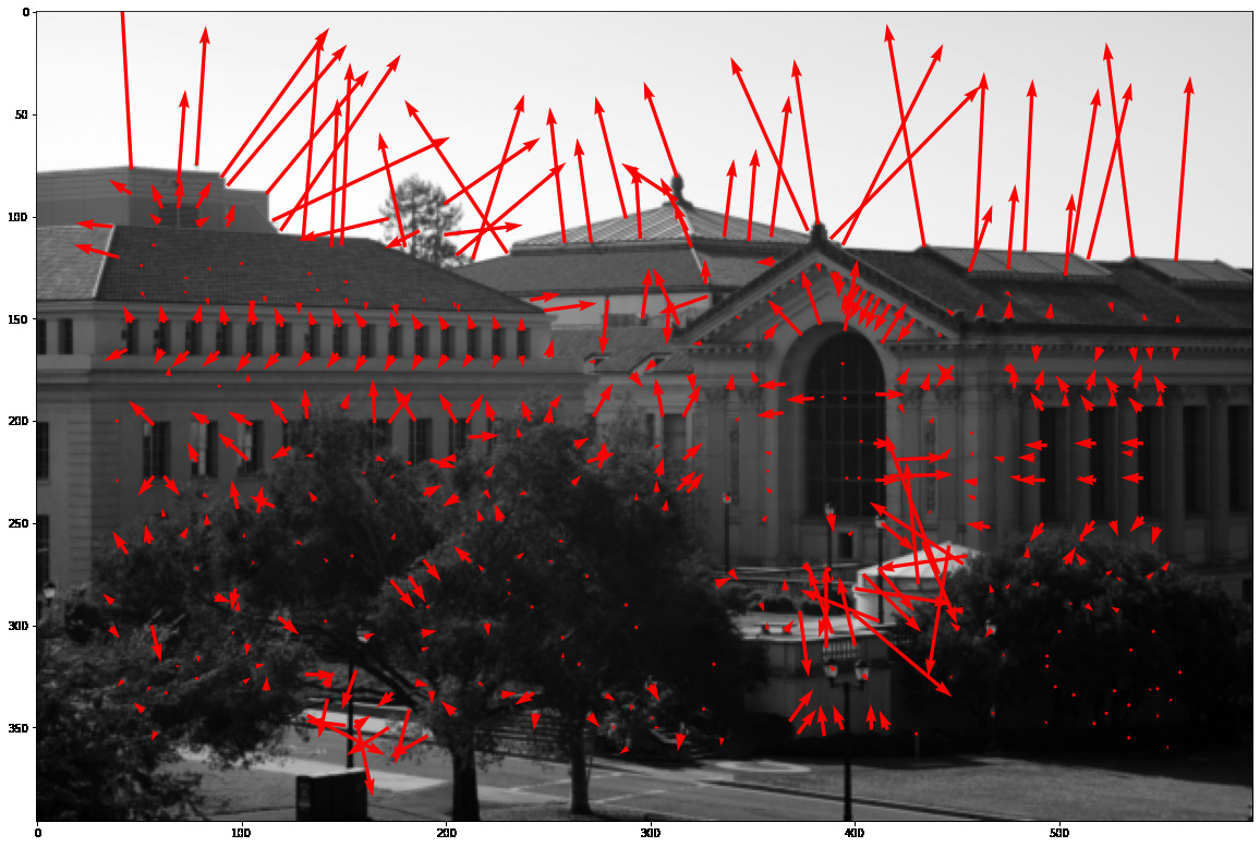
We first use the Harris corner detector to find potential points of interest

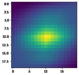
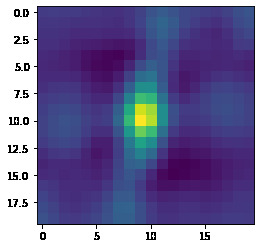
Bell/Whistle: Here we use a gaussian derivative to find a smooth local gradient at each point

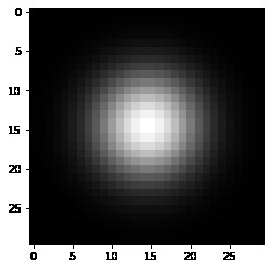
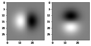
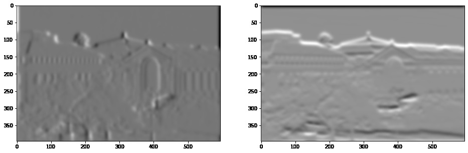
Each point then has a gradient attached to it. Later we will transform our patches such that they are aligned on their gradient.

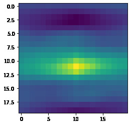
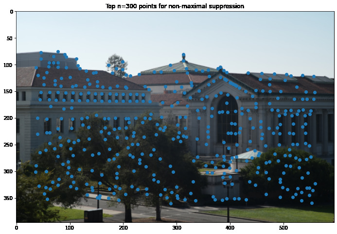
Adaptive Non-maximal Suppression

Next we perform adaptive non-maximal suppression: this thins out the points we select by finding local maxima, giving us a better, more even distribution of points.

Orientation-Invariant Patch Extraction

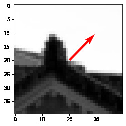
Now we can construct our gradient-aligned feature patches to match between images. The patch is constructed by first building a transformation corresponding to a translation of the origin to the coordinate, a rotation to align the gradient, and then a scaling to sample from a wider area.

Bell/Whistle continued: For the rotation, we have that the normalized gradient is u/|u| = [cos(t), sin(t)] where t is measured relative to the y-axis (since it is the first coordinate). To make the inverse transformation to align by the gradient, we want a rotation by -t. Given cos(t), sin(t) we know that cos(-t) = cos(t) and sin(-t) = -sin(t) so we only need to negate the second term of the normalized gradient everywhere in our formula.

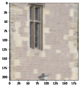
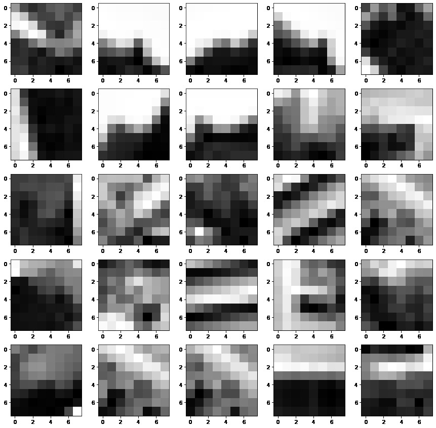
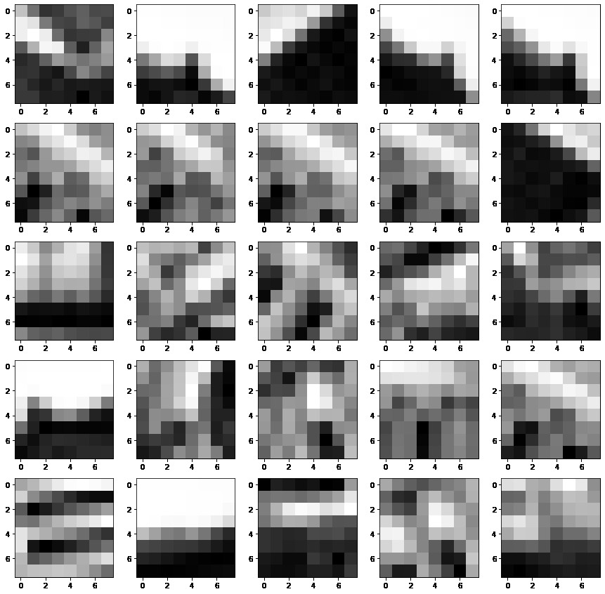
We take an 8x8 grid of points, centered at the origin, and apply this transformation to get their corresponding point in the whole image. We then interpolate these point values from a blurred version of the image to make it resistant to noise. This yields the following patches.

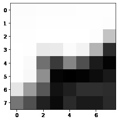
We do this for each image to get two sets of aligned patches

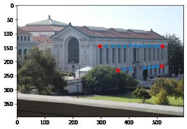
Feature Matching

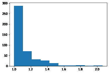
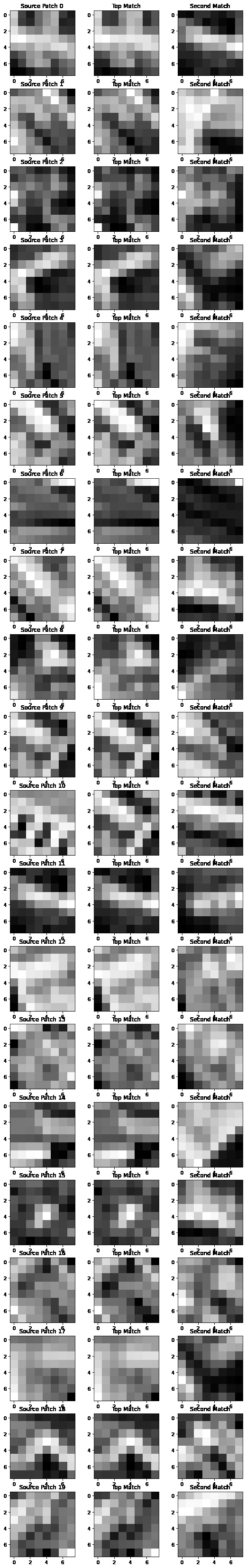
We then compute the normalized cross correlation of each of the patches, and select patches who have a large ratio between their best match and their second best match. This indicates that the patch is a good feature, as it looks like no other feature in the other image.

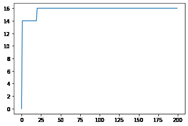
RANSAC

From these matches we can then use the RANSAC algorithm to robustly compute a good homography between our two images.

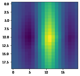
This is the number of maximal inliers v.s. the number of iterations we run for. It converges relatively quickly.

Part A/B Combined: Autostitching

We can now combine these two algorithms to automate the process of aligning images!

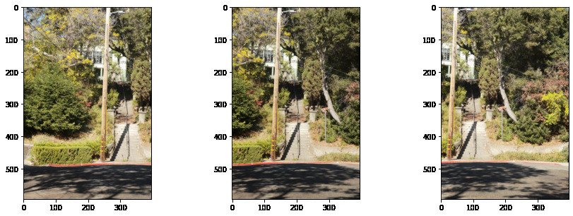
Comparing our outputs, we see our autostitching method performs very well:

Manual	Automatic