We have all used the panoramic function in our iPhones before. In one swift motion, we simply move our iPhone from left to right to capture the entire scene in front of us. However, the implementation of this panoramic image stitching is not so simple. It involves many different mathematical computations to stitch the overlapping areas of the images together.

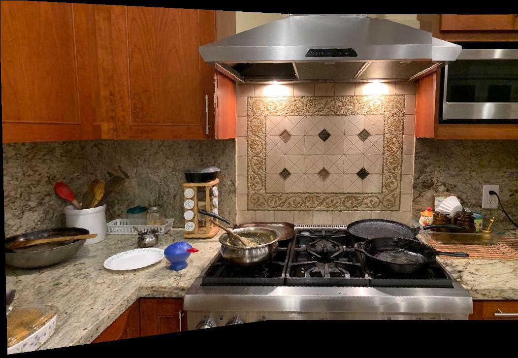
In this part of the project, I manually create mosaics by selecting points on the source and desination images myself. Using these points across both images, we create a homography matrix that transforms the points in the source image to the points in the destination image. Using this homography matrix, we create a warped image that essentially warps the source image to the orientation of the desination image. Finally, we blend the warped image and the destination image to create a panoramic stitching of the two images.
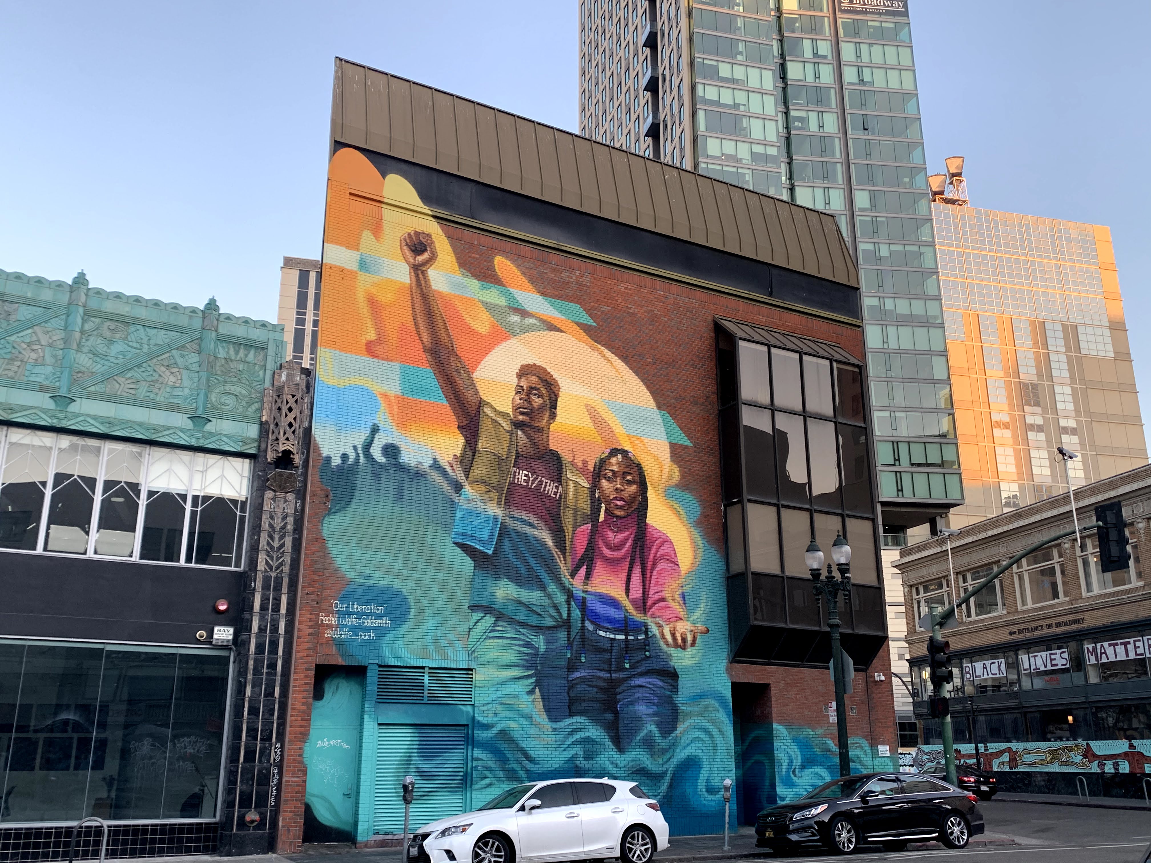
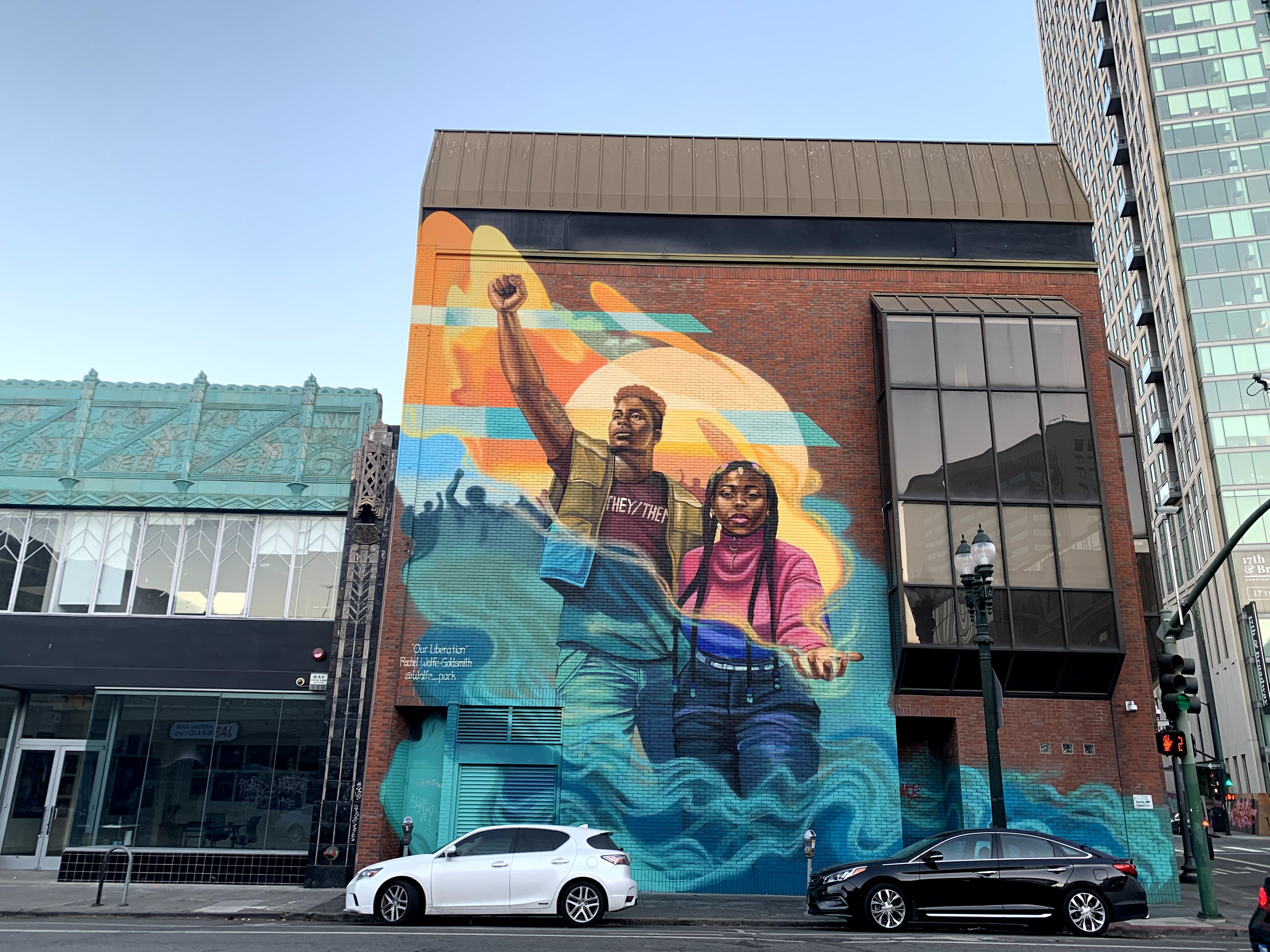
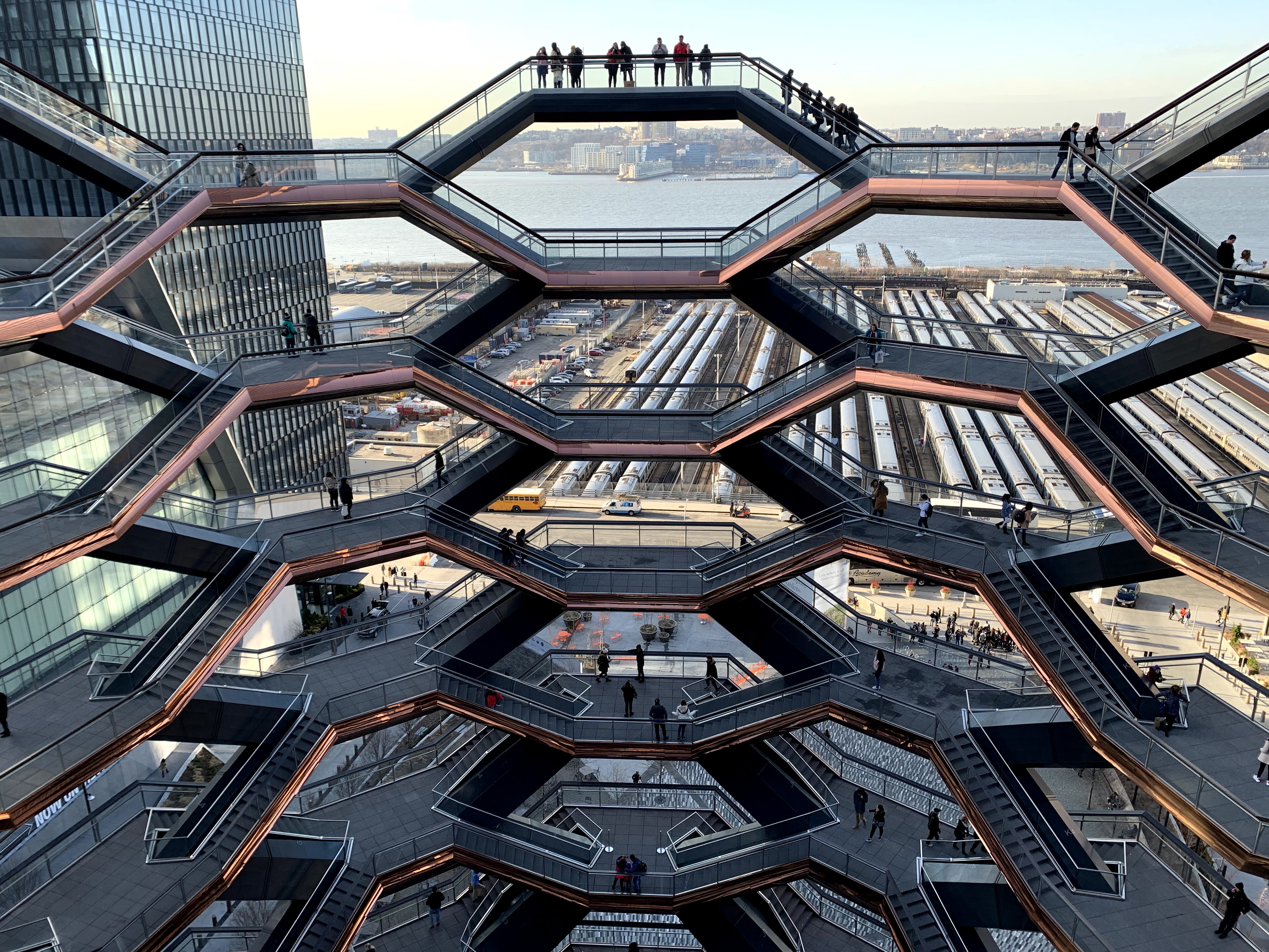
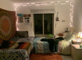
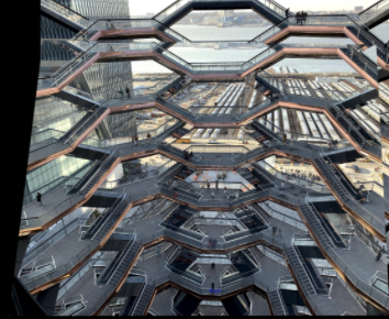
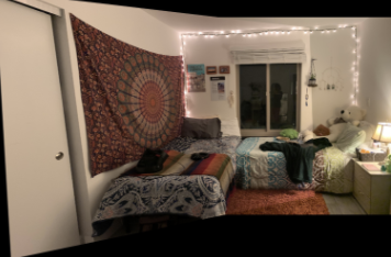
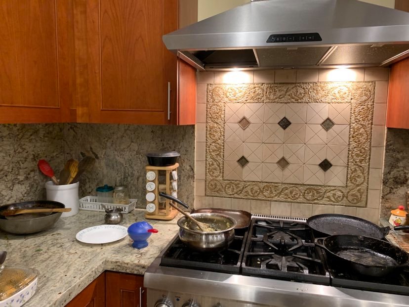
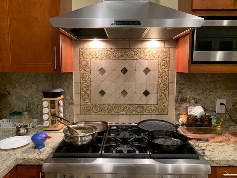
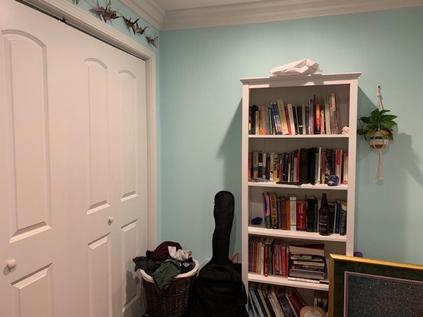
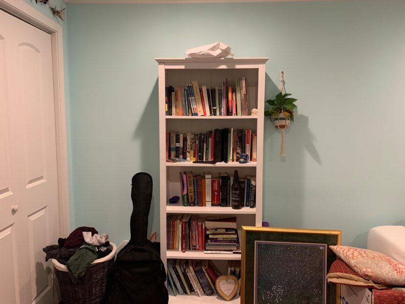
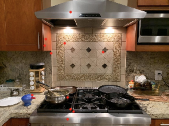
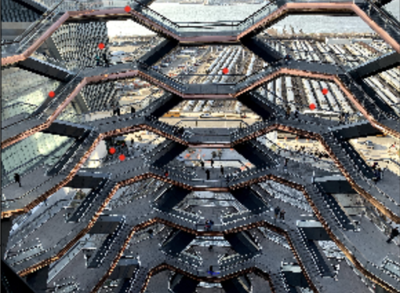
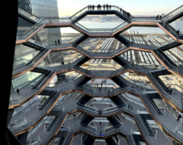
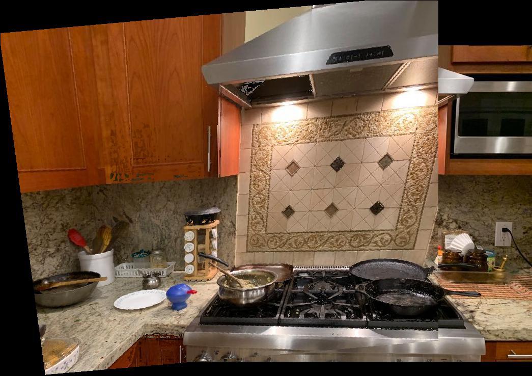
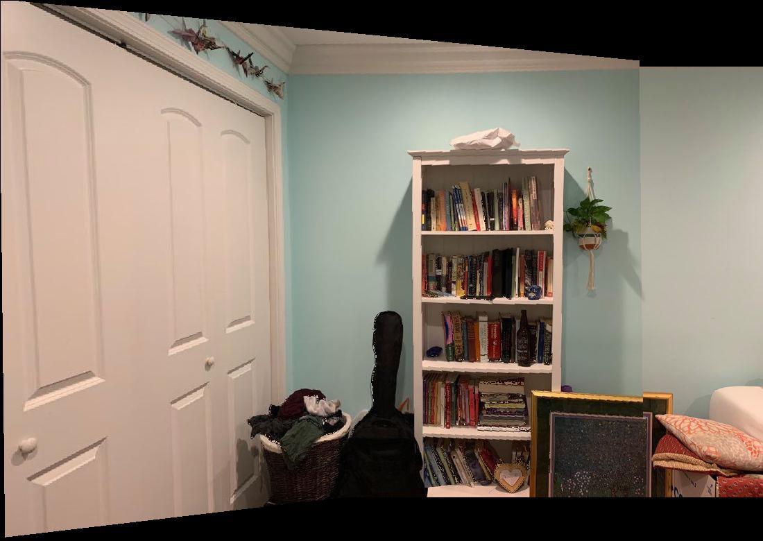
This step is pretty self explanatory. I picked threee different sets of images where the images are taken from different angles.

I selected 12 points in both images to map between the images.
A projective transformation is a linear transformation that warps an images with 8 degrees of freedom. Image projection from a fixed center of projection can be simulated by 2D image warping. In this part, we will compute the transformation matrix between one image to the other. This matrix is called the homography. This 3x3 homography matrix exists such that p' = Hp. Homography preserves straight lines but not parallelism. To find the matrix for the homography transformation, we have to select more than 4 pairs of corresponding coordinates (in my case, I picked 12). After computing this homography matrix, I matrix multiply the homography matrix by the selected points in the image. This results in the warped images (the source image's pixels adapted to fit the destination image). I used a bounding box method, where I created a dummy image that is of the size of the destination image. I apply the inverse of this matrix, H^{-1}, to the dummy image to compute the transformed coordinates onto the source image. If the coordinates are within the bounds of the source image, then you get the r,g,b values at that coordinate in the source image and place it in the dummy image. This dummy image is our warped image.
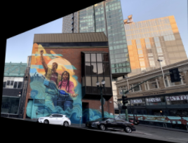
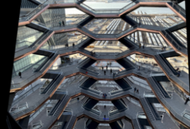
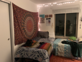
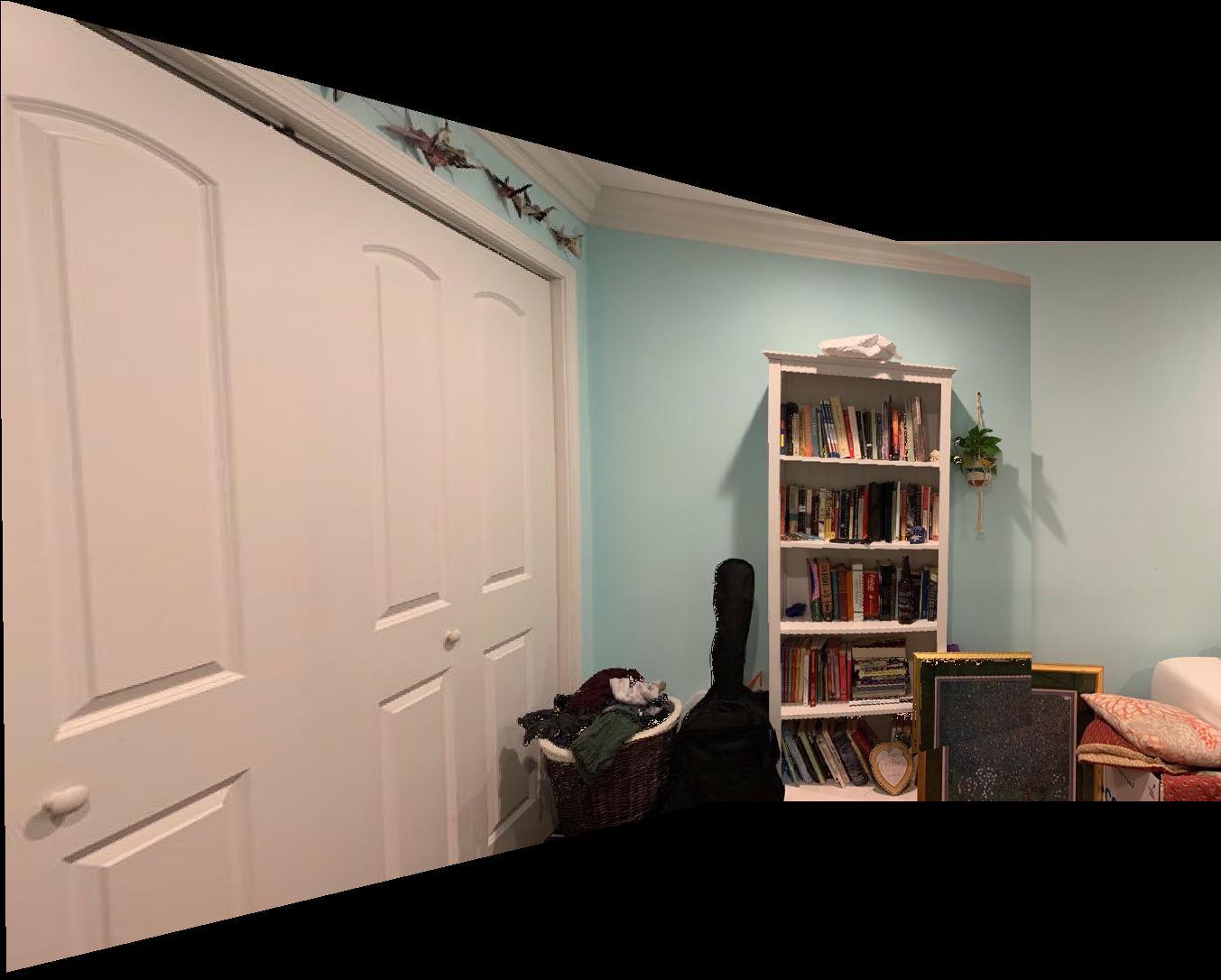
Image rectification is essentially trying to warp an object in an image that we know is a rectangle in reality but is not presented as such in the image due to the angle of the image. In this case, the window doesn't appear as a rectangle in the original image. To rectify an image, I picked four points in the image that formed a square. Then I warped these selected points to four selected points [0 0; 0 1; 1 0; 1 1] that form a square. This rectification is used to test if the homography function works properly. Originally the window was at a slant in the image, As you can see, in the rectified image the window is now shown in rectangular/planar way,
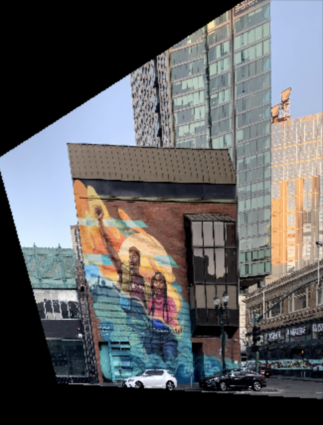
To blend the images, I didn't use the laplacian stack method. Instead, I used a bounding box method. I recreate another image that is of the size of the source image. We iterate through the coordinates in the source image. If the coordintes are in the bounds of the destination image, we check if they're also within the bounds of the source image. If so, we get the r,g,b values from the destination image at those points and place them in our blended image. If they aren't in the bounds of the destination image, but they are in the bounds of the source image then we can again the r,g,b values from the destination image at those points and place them in our blended image. Otherwise, we place r,g,b values of 0 at those coordinates.
The biggest thing I learned was regarding the homography matrix and how to solve for that matrix given selected landmarks. Also I learned that the more points you pick, the more accurate your results. I had to draw many diagrams in my notebooks to visualize the matrices and the dimensions of the matrices to understand how to compute the transformed points.
In the previous part of the project, I manually created mosaics by selecting points on both images myself. In this part, we attempt to automate this process of point selection. This portion of the project is based on the paper "Multi-Image Matching using Multi-Scale Oriented Patches” by Brown et al. The general idea of this paper is to start by selecting a large set of candidate corner points, and narrow this set of points down at each step using various differen measures. At the end, we perform a homography on the final set to create our warping and then stitch our image together
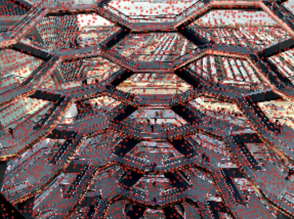
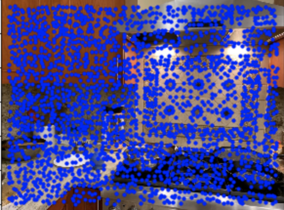
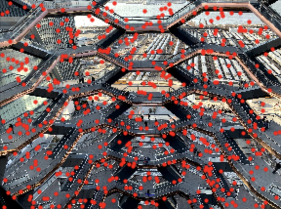
Based on the algorithm in the paper, we choose a huge set of corner features with the Harris Interest Point Detector. This essence of this algorithm is that it scans for big changes in image values when there is only a small shift in a patch. This is a very vague requirement, which allows many points that don't look like corners to be labeled as corners. Since this generates very large amount of points (in the 100000's), the later steps can take very long amounts of time. In order to increase efficiency, I finetuned the paramenters to have a spacing of 30 rather than 1 in the final local maximum function.
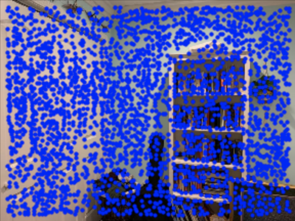
At this point, we have way too many Harris points that are way to close together. This step is used to choose the best of these Harris points and choose them such that they are very spread apart. If we were to simply choose the highest values from our Harris set, we would not get good results because a lot of the points would be close to each other. The Adaptive Non-Maximal Suppression (ANMS) uses the following equation:

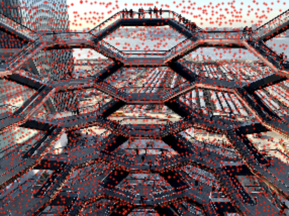
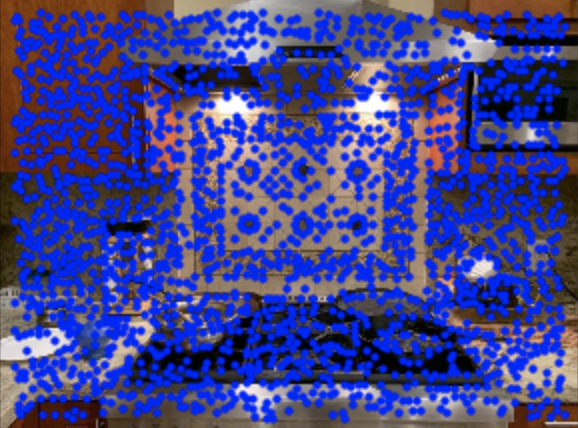
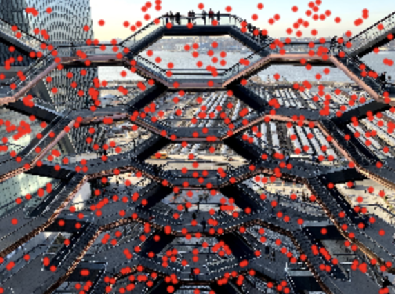
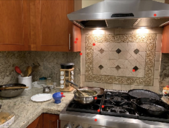
We iteratively create a list of potential points that satisfy the equation above. Using a constant c_robus (I used 0.9 as suggested in the paper), we want to only take points with the largest minimum suppression radius r_i given in the equation. Conceptually what we are doing is selecting points with a high corner strength which are also far away from other points. I pick the top 500 points at the end to select the top 500 potential points with the highest corner strength. As you can see in the images below, there are significantly less points than chosen in the Harris set.

Now we have narrowed down our Harris point set to a more manageable size. However, now we need a way to find the corresponding point in the destination image, given a point in the source image. In order to do this, we create feature descriptors, which are 40x40 patches around an interest point. I applied a Gaussian blur on this 40x40 patch and then downsize it to 8x8 and then normalize it to have a mean of 0 and standard deviation of 1.
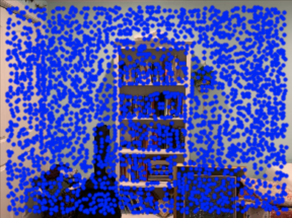
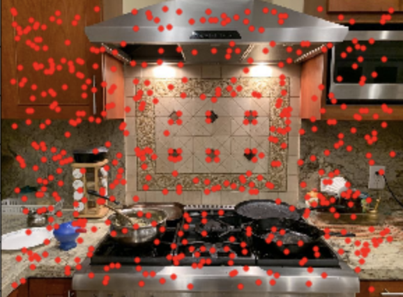
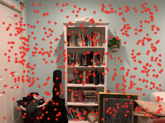
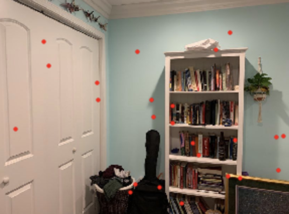
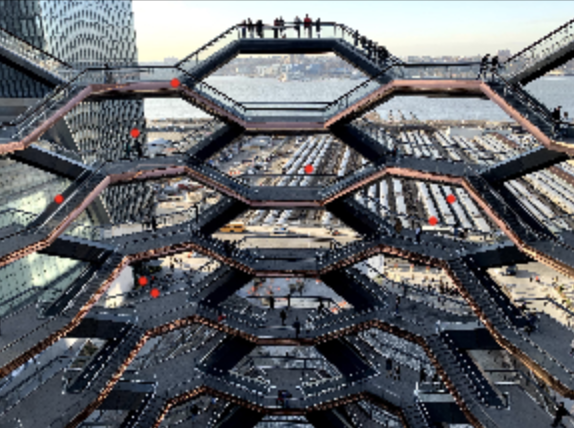
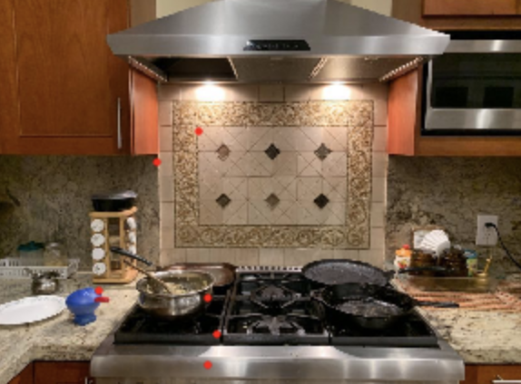
Now we have a sort of comparison metric (set of feature descriptors) for points in both the source and destination images. We use these descriptors to try to "match" these points across the images to find corresponding points. Following the algorithms explained in the paper, I look at each interest point in one image, and compare the distance (the sum of squared error between the two vectors) between its feature descriptor and the feature descriptor of every interest point in the other image. I keep track of the minimum distance and the 2nd-to-smallest distance from the patch in the source image to every patch the destination image. If this ratio of the minimum distance to the 2nd-to-smallest distance is small enough (I used a threshold of 0.3 as suggested in the paper), then I include this as a pair of matching features. Conceptually, if two points are corresponding, then they should be closest in feature descriptors. As you can see in the images below, most of the red dots match up in the objects they are pointing to (barring a few outliers).
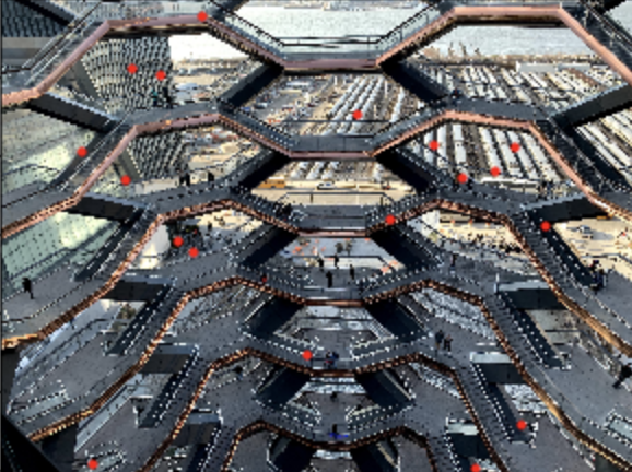
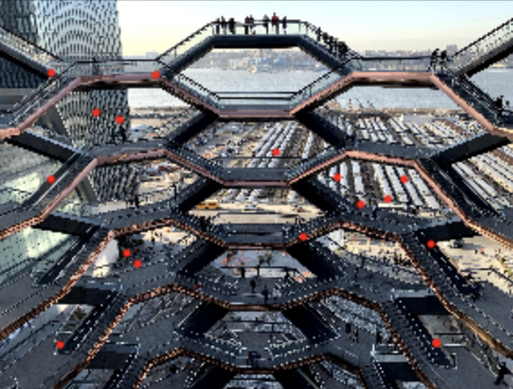
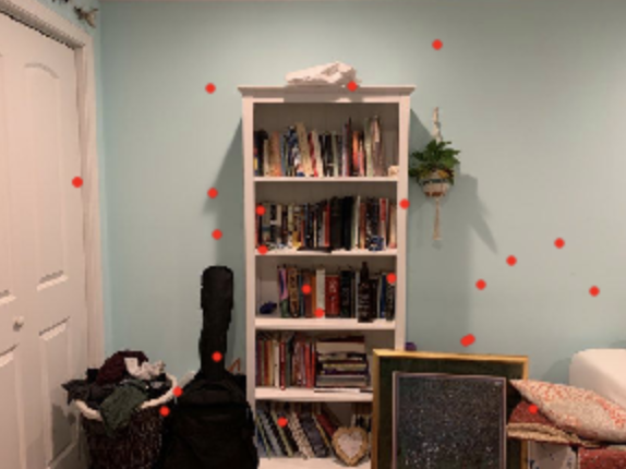
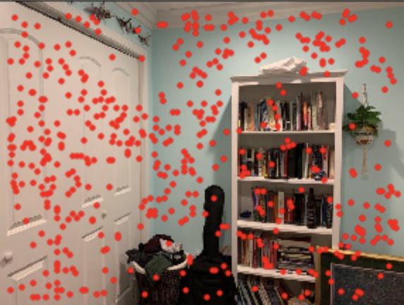
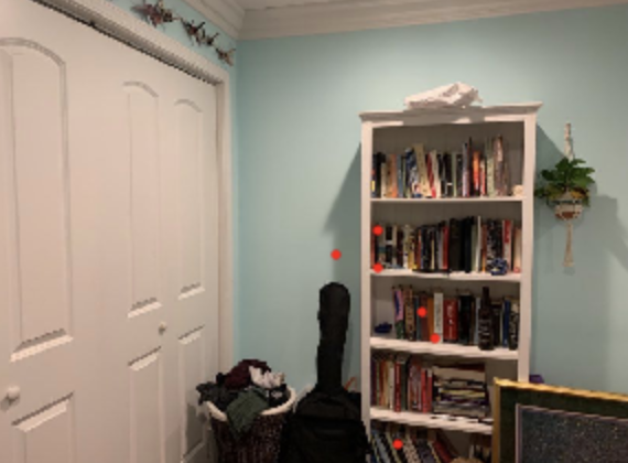
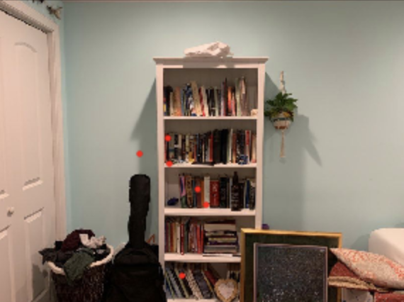
As seen in the feature matching points, there are few outliers where the points do not match up. We use the Ransac algorithm to get rid of these outliers. Ransac is an iterative algorithm where we randomly sample 4 of the pairs of feature matched points. Using these 4 pairs of points, we can compute a homography matrix H. Next, we apply H to the set of feature-matched points in the source image to transform it to predicted destination points. We compare predicted destination points to its corresponding feature-matched point in the destination image. If this error is small enough (less than some epsilon between 1-5, varies on the image), we count this match as an "inlier". An inlier is a point that agrees with the homography matrix H generated by our sampled points. We repeat this algorithm for many iterations (I chose 10000). We keep track of the Hmatrix that has resulted in the largest set of inliers. The last step is to take these two largest sets of inliers (from both the source and destination images) and compute a final homography matrix H, which should give us the most accurate H matrix. As you can see in the images below, the points match up very precisely.

In working on the second half of this project, I learned just how complicated the panoramic stitching function in the iPhone is. This half of the project took a lot of conceptual planning and thinking before even attempting to begin coding the functions. I learned that conceptual research papers describing algorithms can be very difficult to interpret and difficult to actually implement. It requires a lot of diagramming and thinking in terms of how to use these algorithms in practice.
