Defining Correspondences
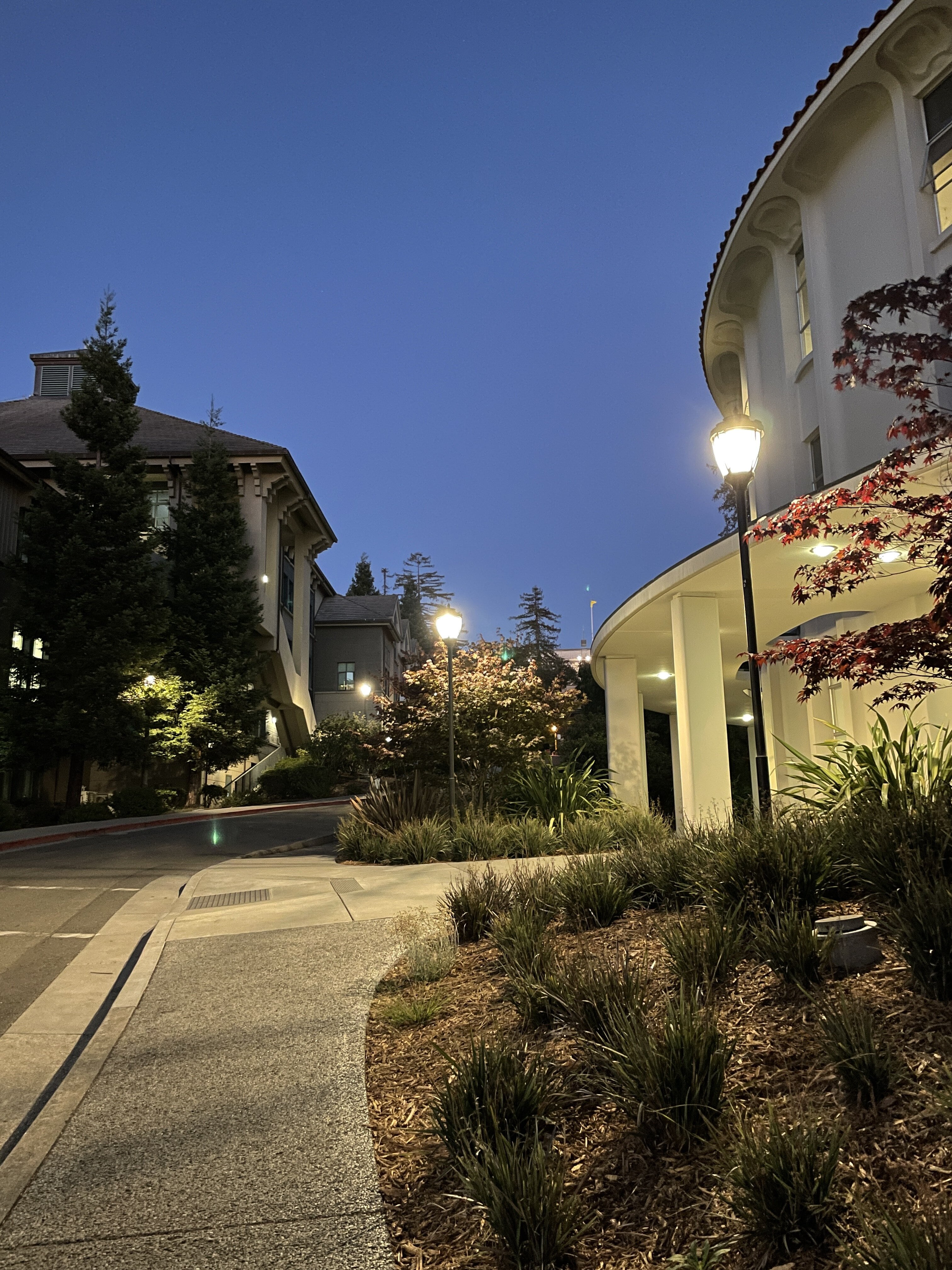
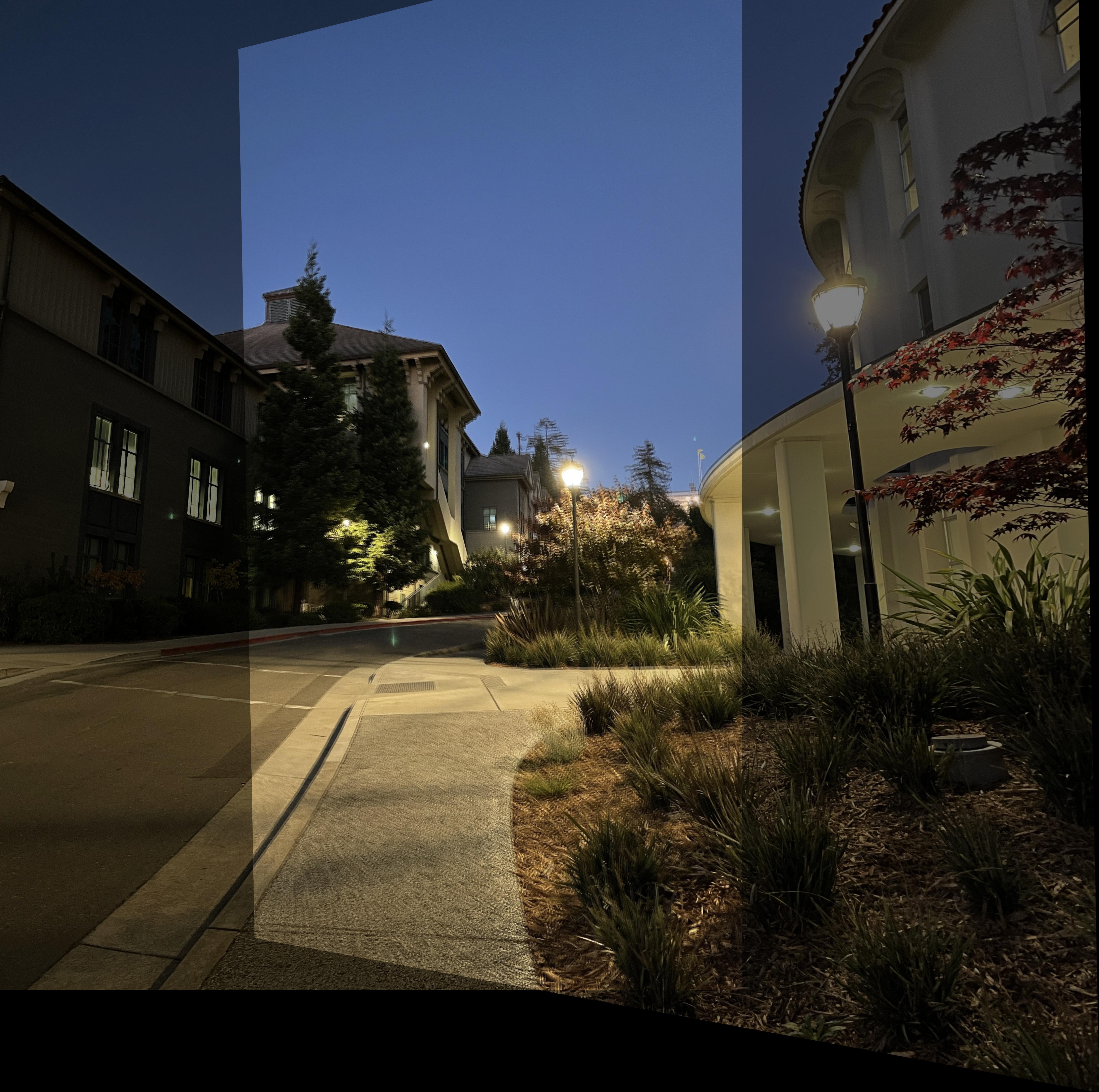
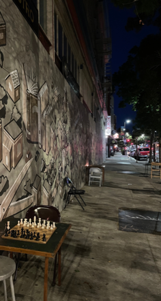
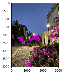
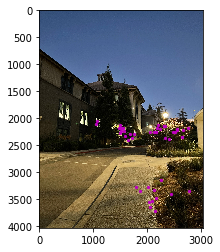
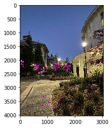
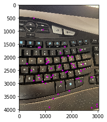
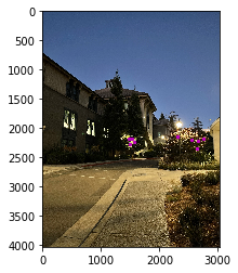
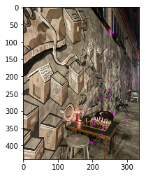
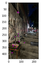
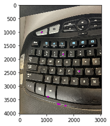
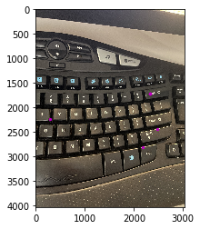
For this part, I used matplotlib's ginput() function to select the set of features that I would use to correspond the two images that would morph to create the panorama. I defined these points on paper, so that I could remember the order in which they were selected. To select the points, I focused on features in the shared region of the two images that stood out (e.g. corners, tops of trees, etc. ). Once I found the points, I saved the feature sets as CSV files so I wouldn't have to reselect them every time.
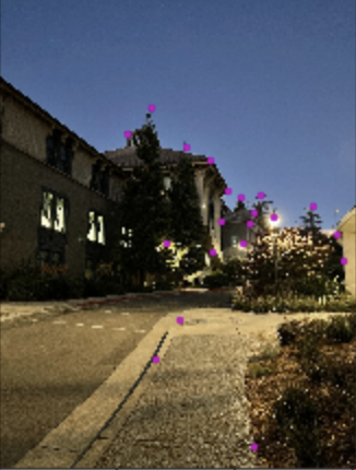
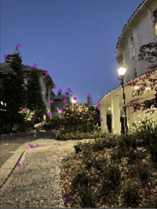
Above you see an example of the feature sets for a collection of photos that will be later blended together for a panorama.
Recover Homographies
Homography is defined as p'=Hp where H is a 3x3 matrix w/ 8 degrees of freedom (lower right corner is a scaling factor set to 1). We find the H matrix by using the correspondence points found earlier. We setup a linear system of equations of the form AH=b where b is the target points. We want to overconstrain the system, so we define more than 4 points in each image. Once we've setup the linear system, as defined above, we solve it using Least-Squares.
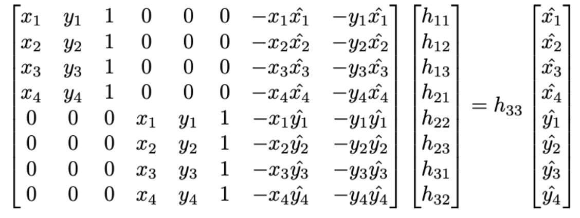
The following site was a terrific resource in guiding this process.
Warp the Images
Here is where we use the Homography matrix, H, previously calculated to warp one of our images so we can blend the collection together.
This is similar to the previous project, but we are no longer doing an affine transformation. Rather, this is now a projective transformation.
The steps to warp the image are as follow:
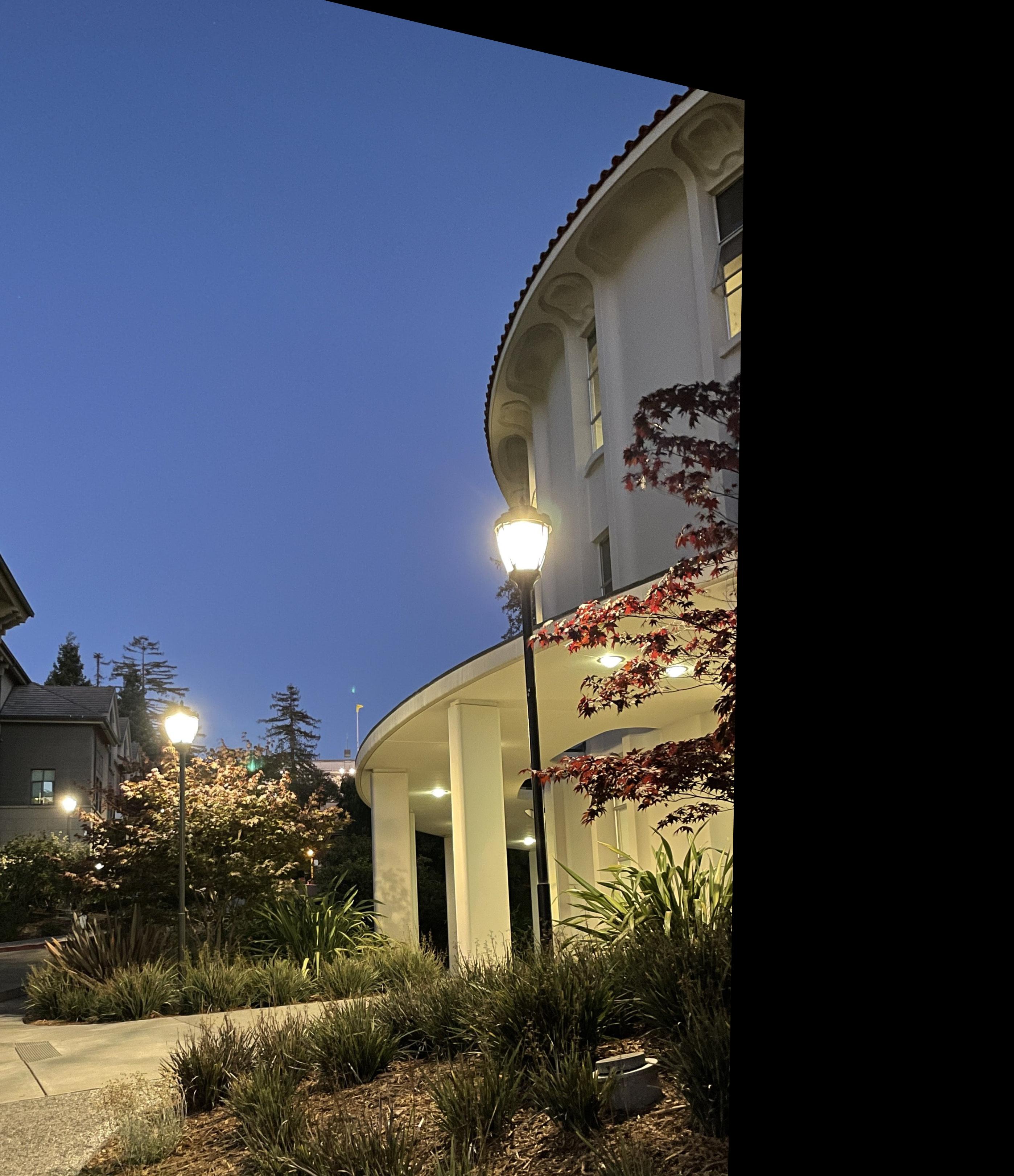
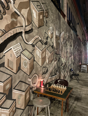
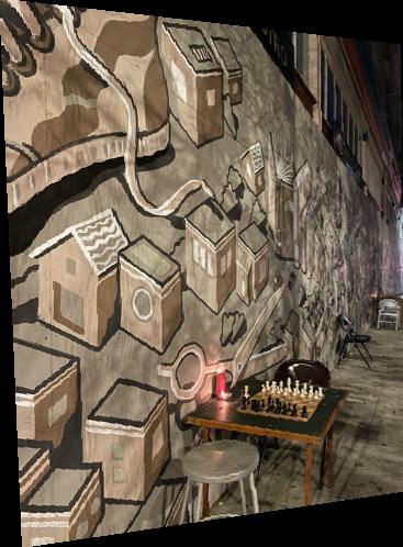
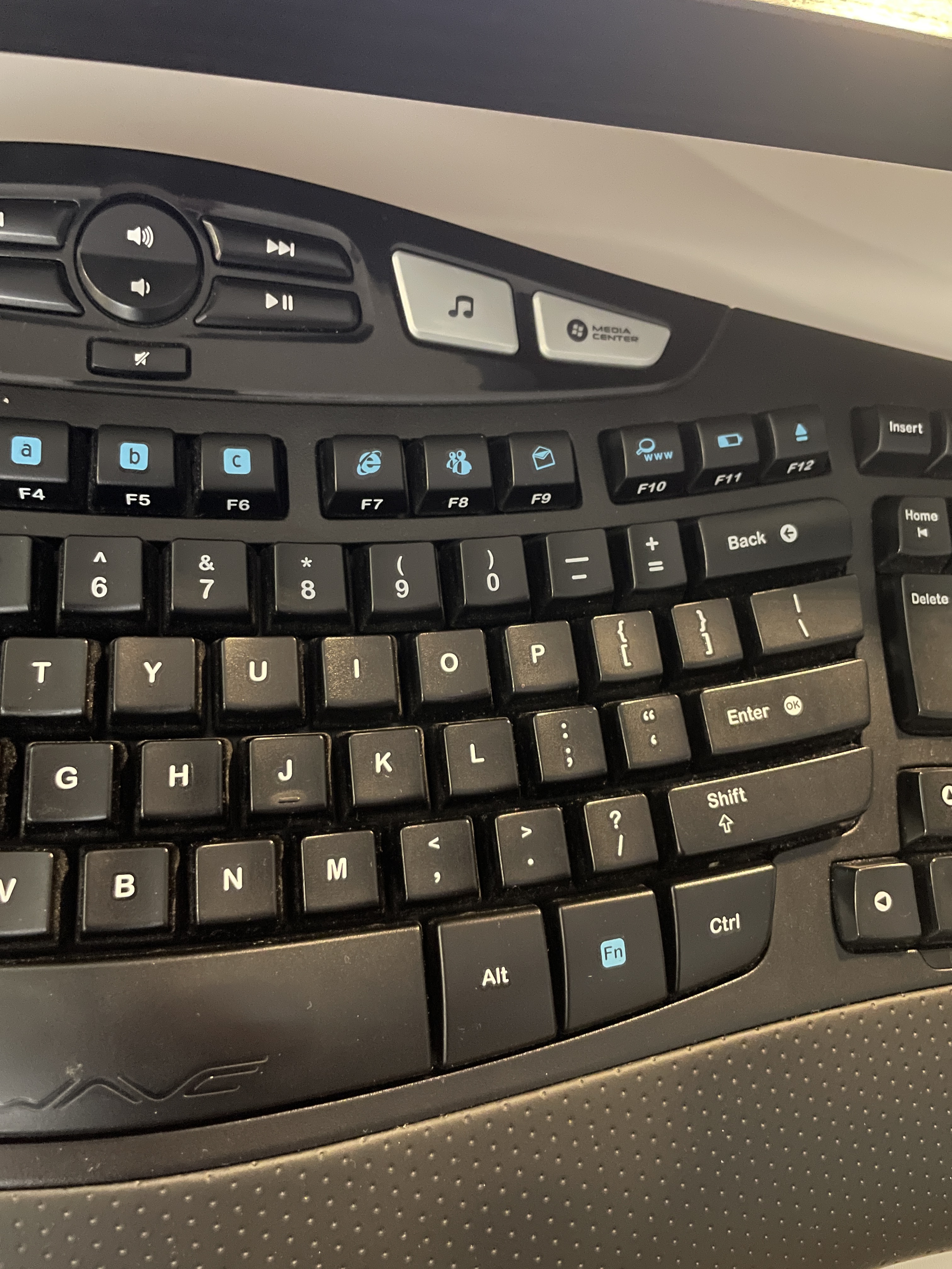

Image Rectification
A bit of a detour from the earlier part of the project, here we are attempting to rectify images. This means we take an image and warp it such that we are viewing it "head-on" (there are examples below). To rectify an image, we follow a similar process as above (the warp process). However, a key distinction here is that we are not warping our image to another image. Instead, we are "straightening" it so that the corners are aligned in a way that we can view it "head-on". To do so, I created an array manually that contained the "warped corners", or in other words, the straightened corners. This was the only difference, beyond that the process was the same as earlier: we define correspondences (in this case we only needed 4 - the corners of the object) and then take the steps described above to warp the image (this time to the straightened corners).


Mosaic
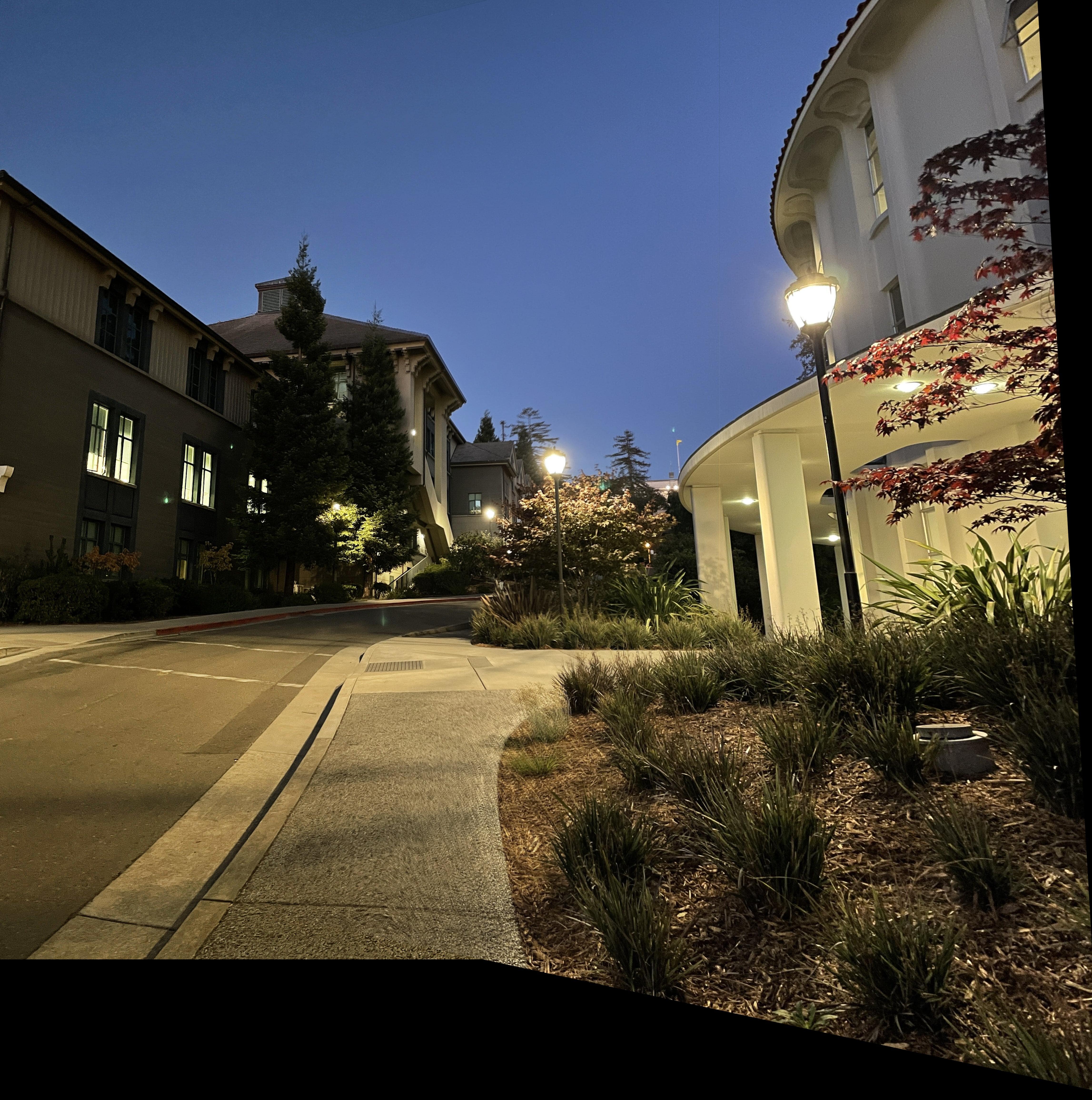
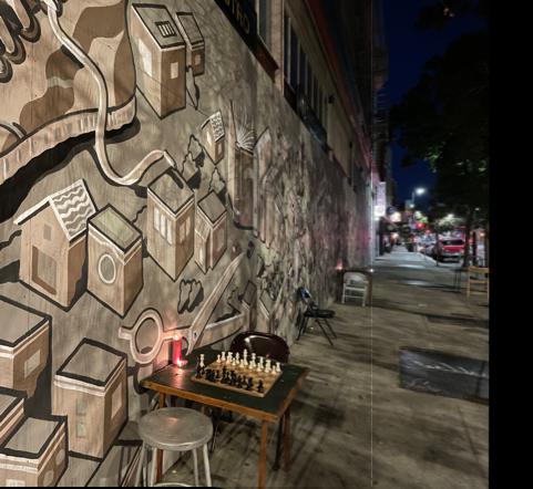
Here we put it all together, we combine our warped images and original images together to create a mosaic of the scene. The mosaic construction process is as follows:
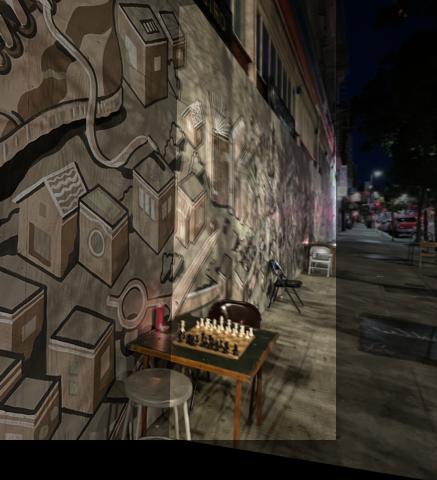
One thing to note, you may notice that the overlapping region between the two images is brighter than the surrounding image. I wasn't able to figure out why this kept happening, I suspect somewhere in my mosaic code I am adding this overlapping region twice and thus amplifying the intensity of the pixels. I couldn't figure out a solution in time and so I decided to put a fix on the backburner until later. If you view the images in grayscale though, it looks perfectly fine :)
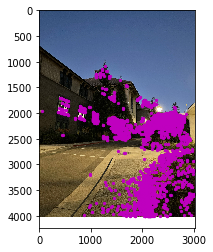
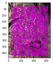
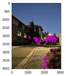
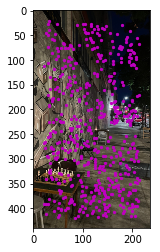
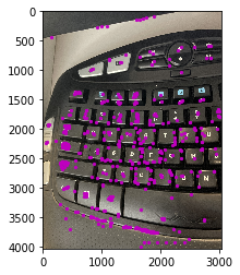
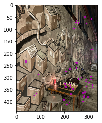
Detecting Corner Features
For this part, I used the starter code function "get_harris_corners.py" to retrieve the Harris corners and their respective corner strengths. One tweak I did make was to introduce a threshold as a parameter to the function as a way to limit the number of points returned (I aimed for ~5k points for each image).

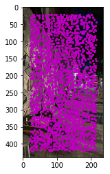
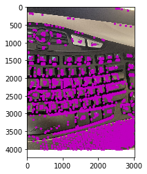
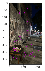
Implement Adaptive Non-Maximal Suppression (ANMS)
Now, we'd like to further limit the number of corners by only retaining those that are a local maximum. More explicitly, for every corner xi, we calculate ri as follows (where xj is some other "neighboring" corner):

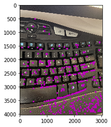
Extract Feature Descriptors for each Point
At this point, we extract a description of the area around our point as a way to efficiently and reliably match features across images. We start by convolving the image with a Gaussian to blur it, this is done to avoid aliasing. Now, for each point:
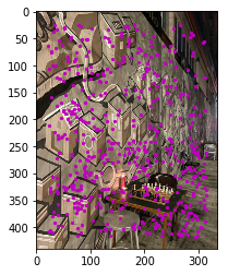
Match Feature Descriptors Between Images
Once we've extracted the patches, we match them between images to create a correspondence. We find the Nearest Neighbor (nn_1) and the 2nd Nearest Neighbor (nn_2), compute the SSD between our current patch and each of those (yielding e1_nn and e2_nn). Finally, we find the "Lowe Ratio", defined as e1_nn / e2_nn. If the Lowe Ratio is within some threshold, then we add it to our list of matched features.
Use RANSAC to Compute Homography
Once we've found the correspondences between features in images, we need to further prune the feature sets and find the "inliers". This is where RANSAC comes in. The RANSAC algorithm is defined as follows and is used to estimate the homography matrix.

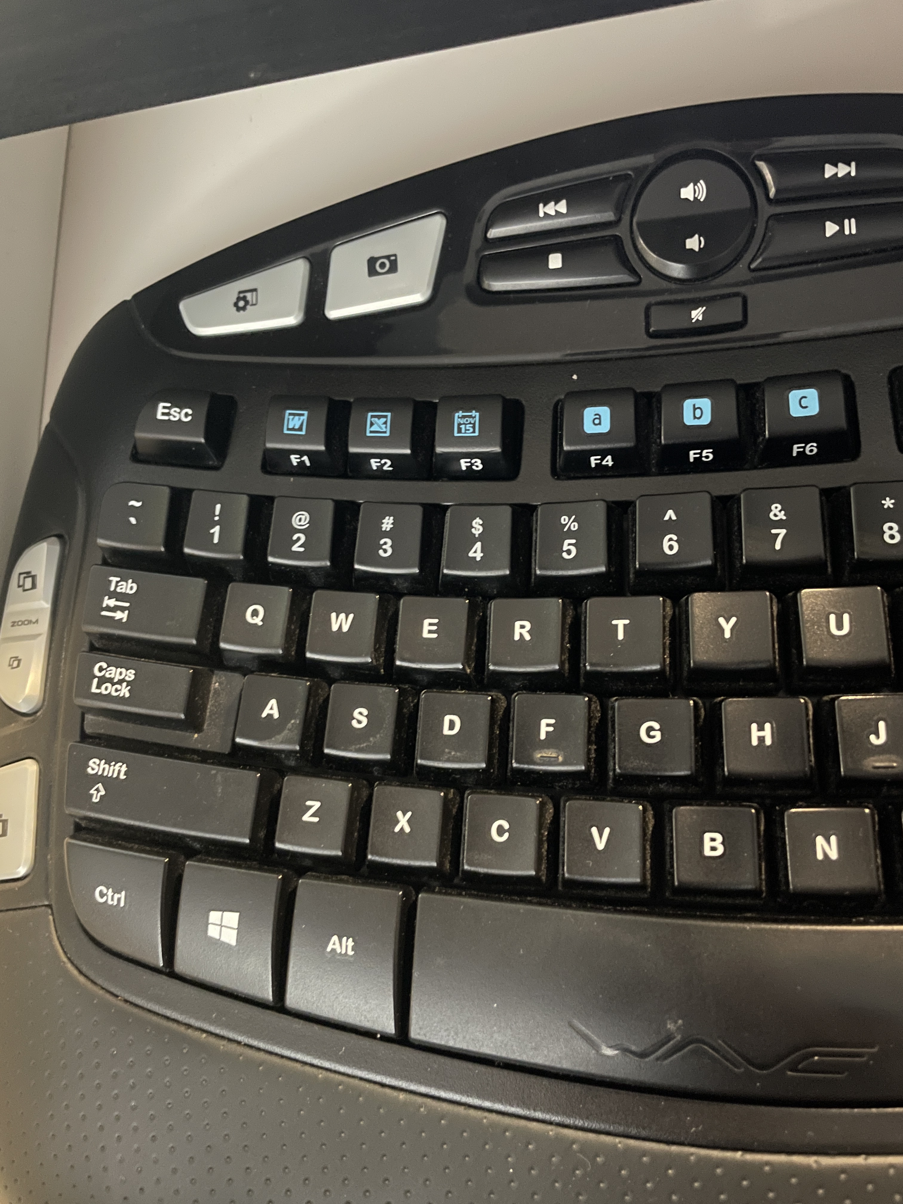
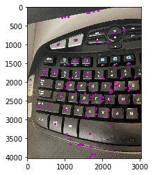
Produce Mosaics
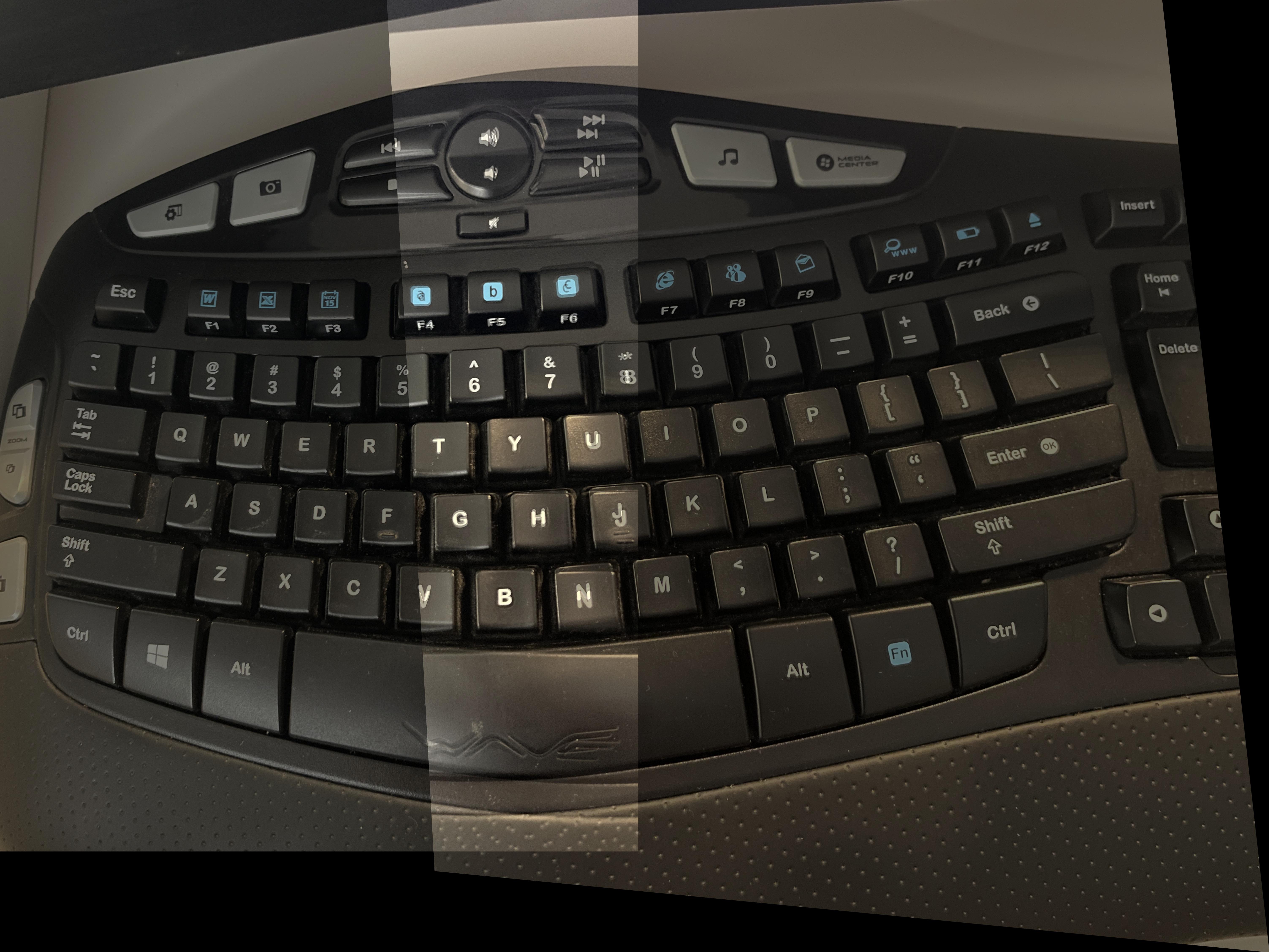
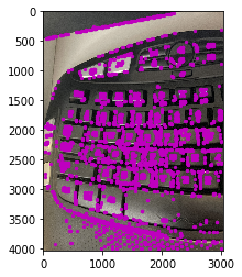
Finally, we put it all together to, once again, stitch together images to create a mosaic. We follow a similar procedure to earlier, but this time all of our features have been automatically selected! The comparisons between the two are highlighted below:
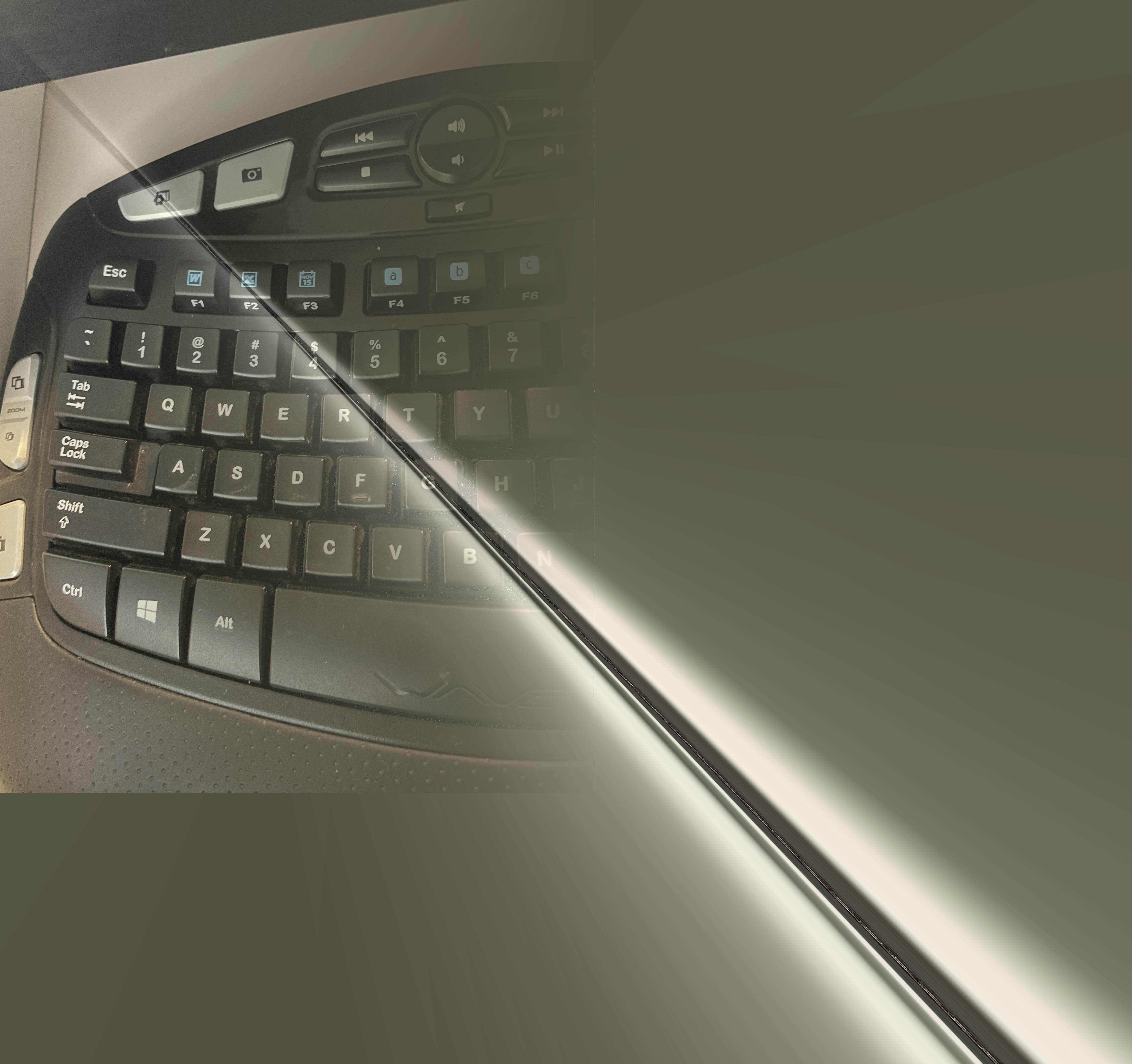
Note: For keyboard auto-mosaic, there is a wedge artifact that slices through the image. This is a side-effect that sometimes occurs with the alpha-blending strategy I used. To eliminate this, I would use a Laplacian Stack to blend the two halves together instead.
What I've Learned:
The coolest part of part A of this project was the image rectification, I found it really cool that we were able to warp our perpective of an image from looking at it at an angle to directly head-on. I can see how this type of transformation would be especially useful for computer vision algorithms that need to analyze bank statements, driver's licenses, passports, etc. Since the user could upload an image that may be crooked, but you'd still be able to extract the key information as if it were taken straight on.
The coolest part of part B of this project was the fact that we could develop code to automatically parse through images and identify the key features that would then be used to (quite accurately) estimate the Homography matrix that is then used to warp and stitch together the images, streamlining the whole panorama-creation-process tremendously!