
To be able to eventually stitch two images together using projective transformation, the two input images should be taken either from the same viewpoint in different directions (with significant overlap), or taken from different viewpoints of a planar or far-away object.
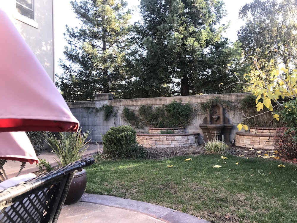
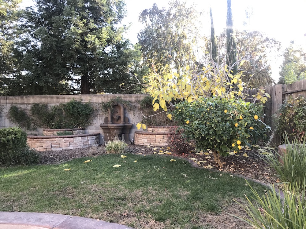
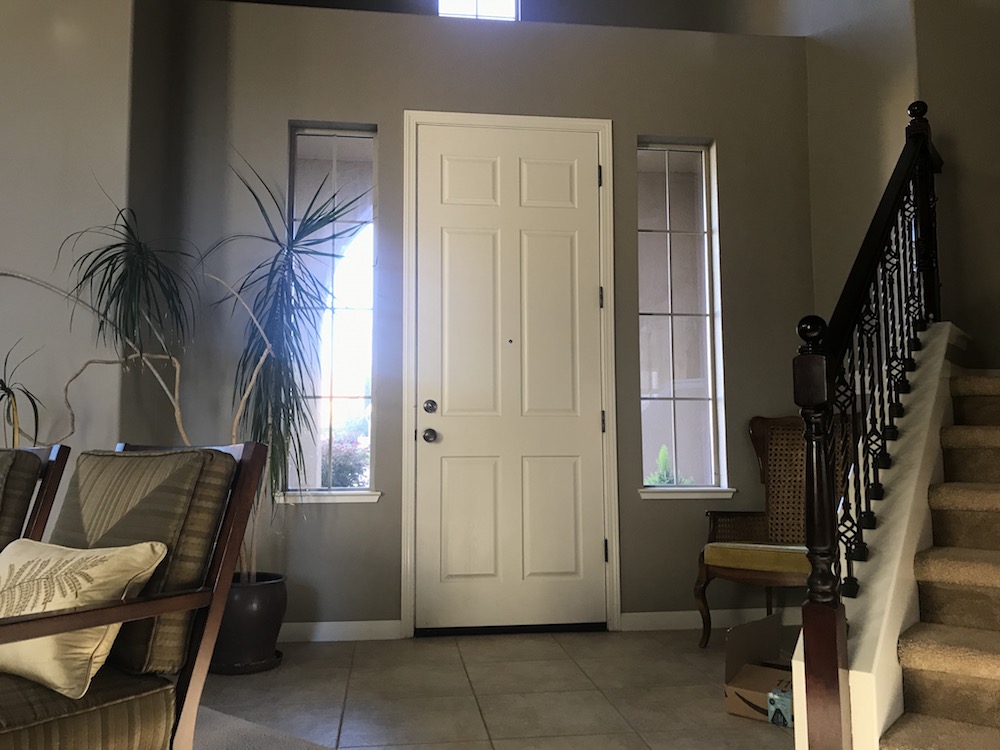
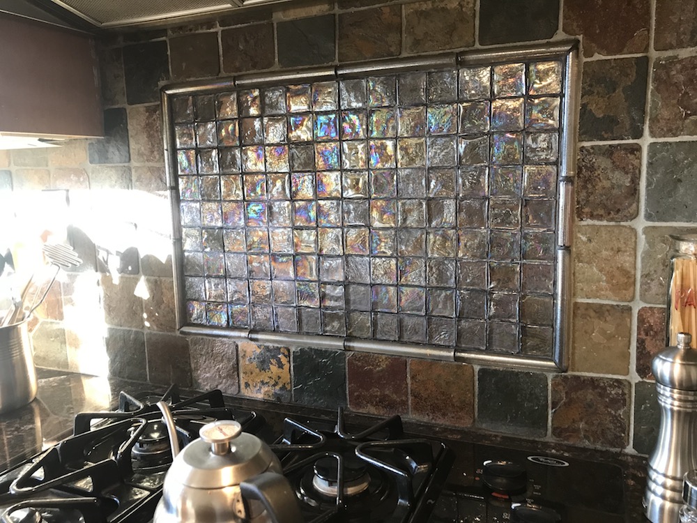
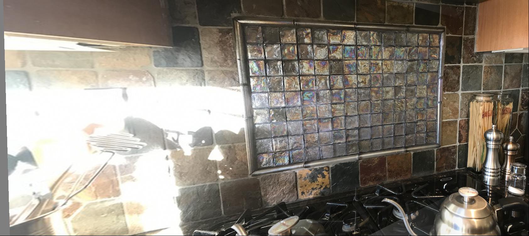
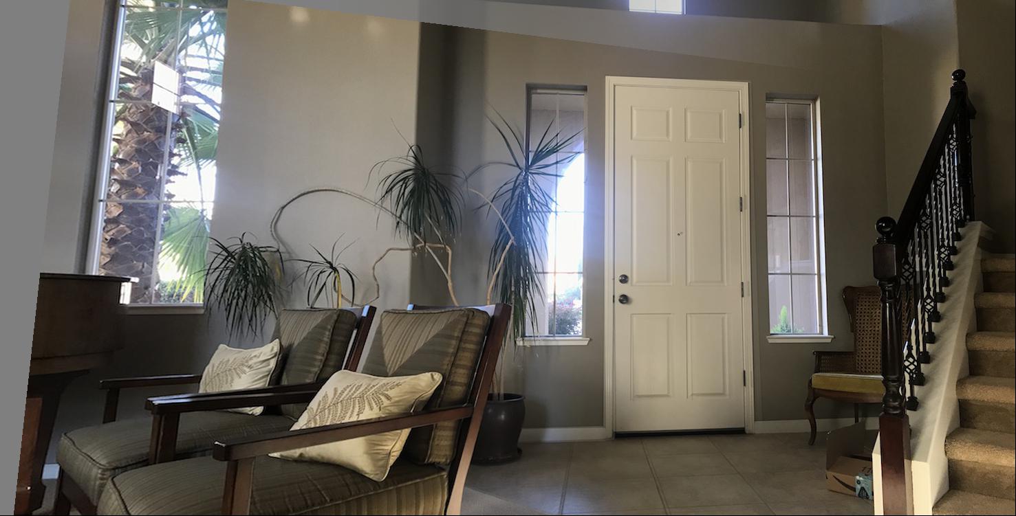
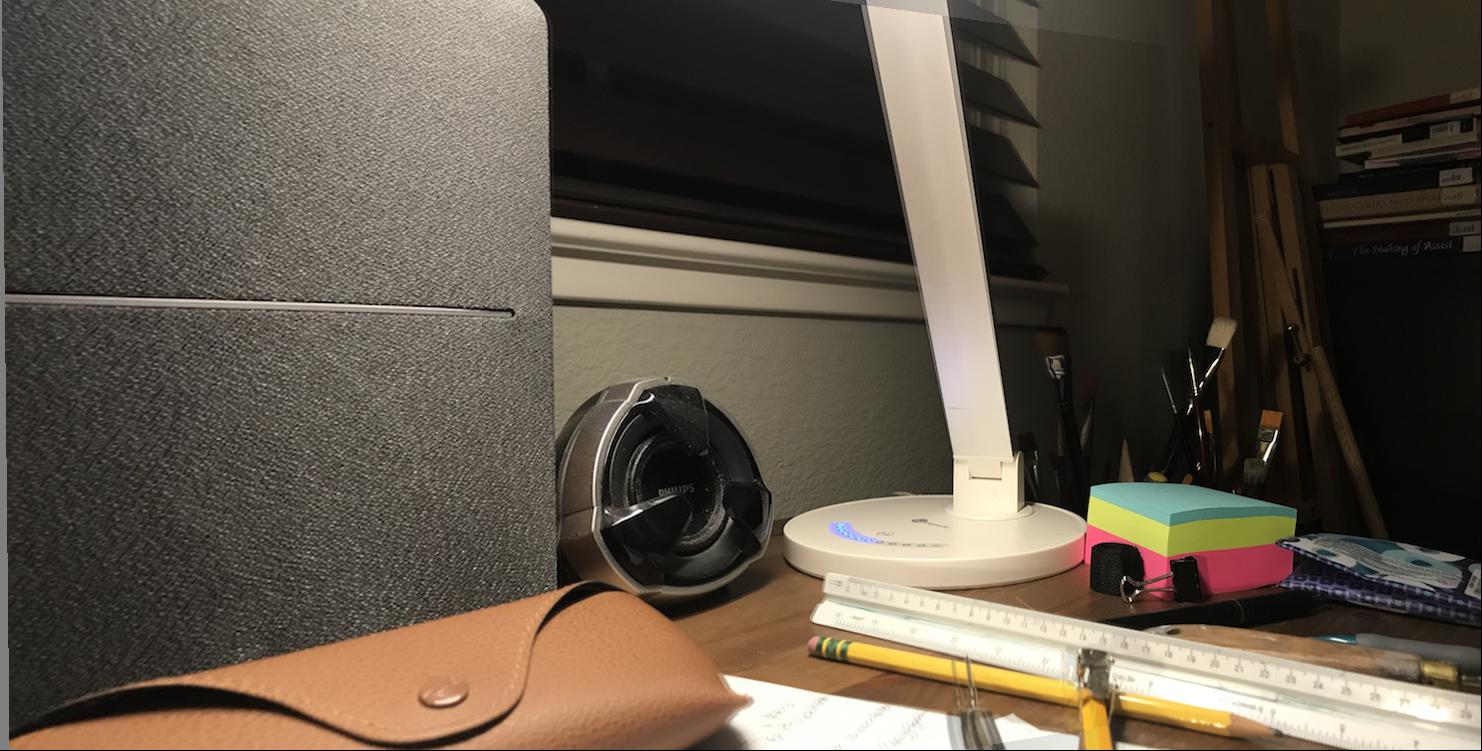
As an example, I took the following two images from the same viewpoint in different directions:
We can represent the homography transfomation as
p' = Hp
where p' is the vector of tranformed points and p is the vector of input points. We define correspondences p and p' by using a UI to capture keypoints via mouseclick on the 2 input images. The matrix H is a 3x3 square matrix containing [[a,b,c],[d,e,f],[g,h,1]], the 8 projection parameters followed by a scalar (1). To compute H, we need to set up an equation of the form
Ah = b
where h is a vector containing the 8 projection parameters for which we need to solve either using a standard system of lin. equations (if we have defined 4 correspondences = 8 points, giving exact amount of equations required to solve for the 8 variables), or least squares (if we have more than 4 correspondences). Our b is just our N (x, y) pairs from the first input image. A is an Nx8 matrix containing the coeffecients of our system of linear equations, the rows of which are [x, y, 1, 0, 0, 0, -x*x', -y*x'] and [0, 0, 0, x, y, 1, -x*y', -y*y'] for each of N pairs.
In my setup, I obtain 8 correspondences (= 16 points/equations) and use least squares to solve for h in Ah = b. Then I simply plug the values of h into the 3x3 matrix H to recover the homography.
For image rectification, the goal is to take one image of a planar object at some viewpoint, and apply a projective transformation to allow the planar object to appear parallel to the image plane. This involves defining one set of kepyoints at the corners of the planar object, rather than a set of keypoints. We then create a corrensponding set of points based on the input points and a scalar value parameter, which determines the w:h ratio of the planar object.
I first sort the input points to determine the top left (tl), bl, tr, and br points. I then fix the top point of the longer height (left/right), and compute the other three points based on that height, for example:
[new_tl, new_bl, new_tr, new_br] = [(tl_x, tl_y), (tl_x, tl_y+height), (tl_x+height*scalar, tl_y), tl_x+height*scalar, tl_y+height)]
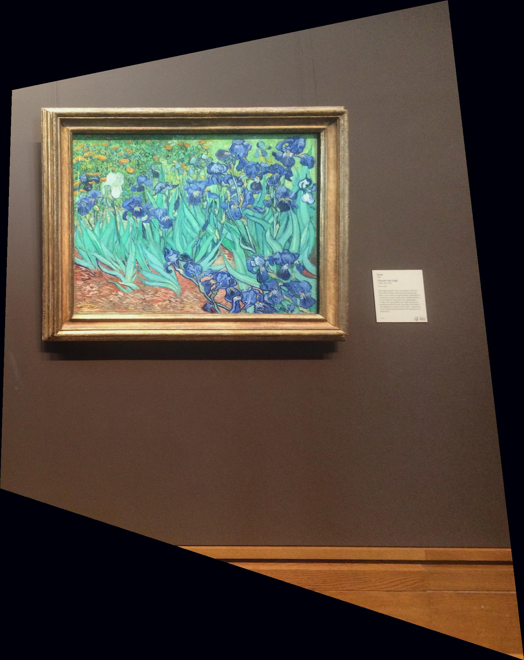
This method is perfect for when you want to photograph of a popular picture at a gallery and you just can't get a frontal view! As an example, I used this photo of Van Gogh's Irises I took a while ago at the Getty Museum:
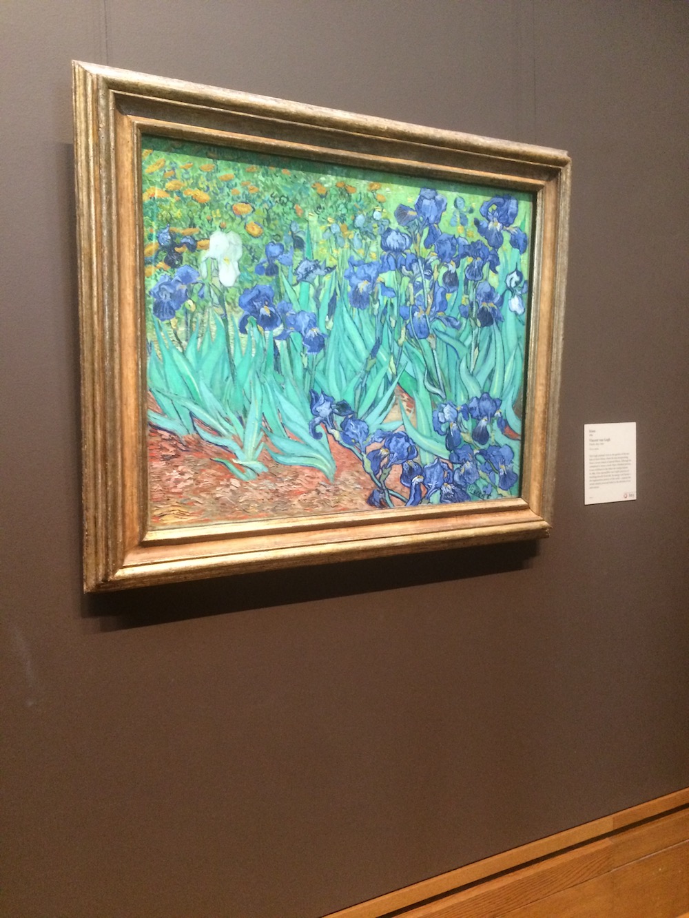
input image
rectified image
The picture on the right looks as if it were taken from directly in front of the painting with no one else around, when in reality there were some people standing in front of the painting also taking pictures! Here are a couple more examples:
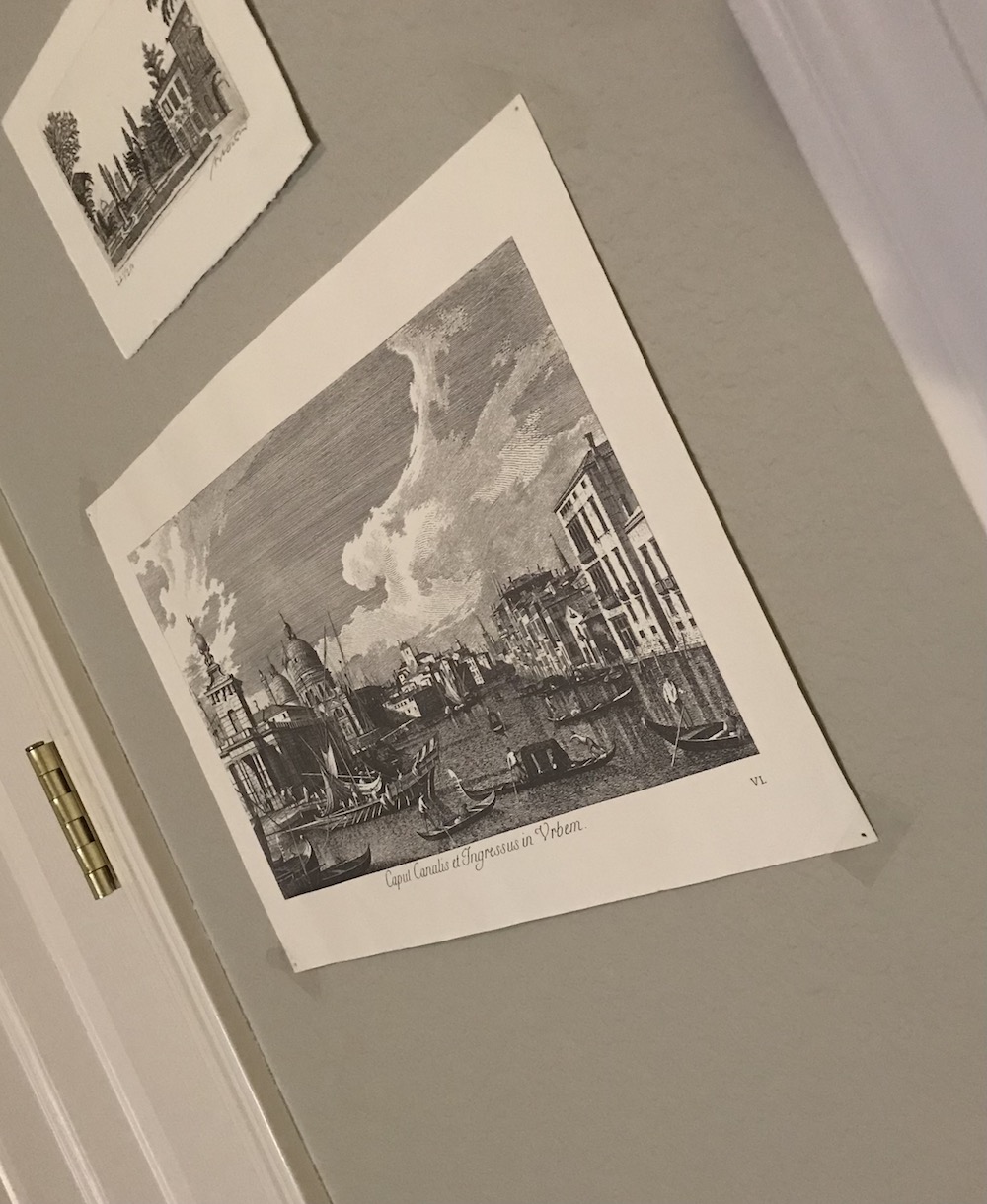
input image
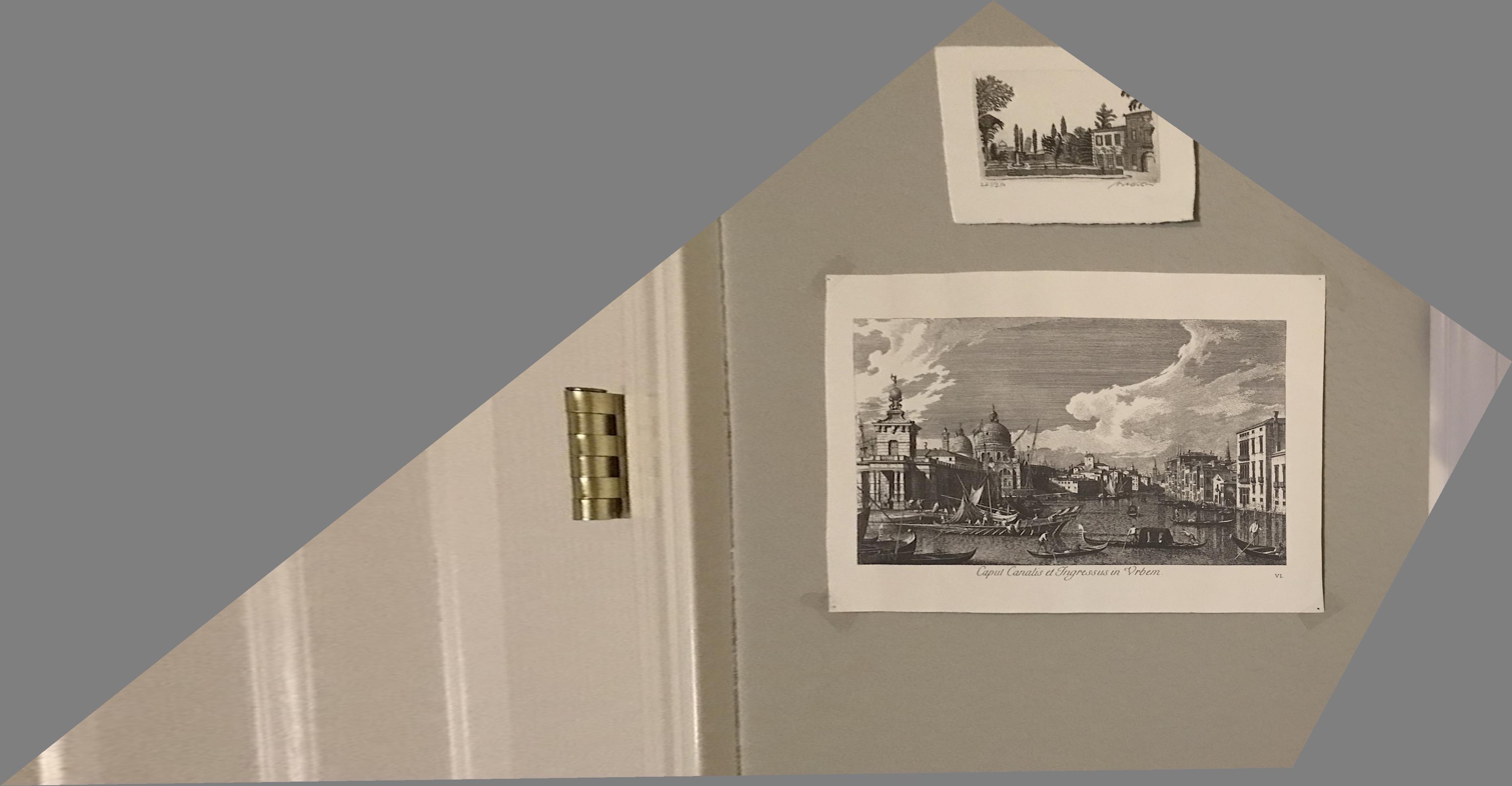
rectified image
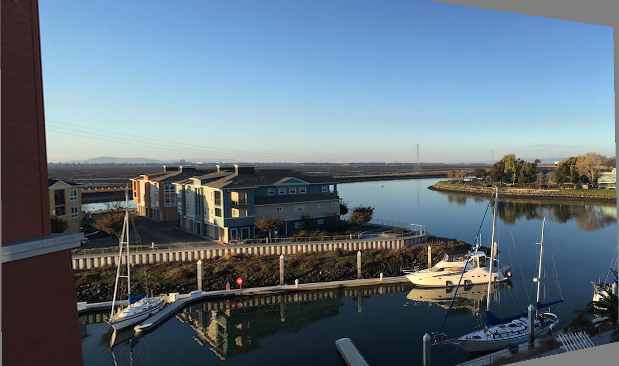
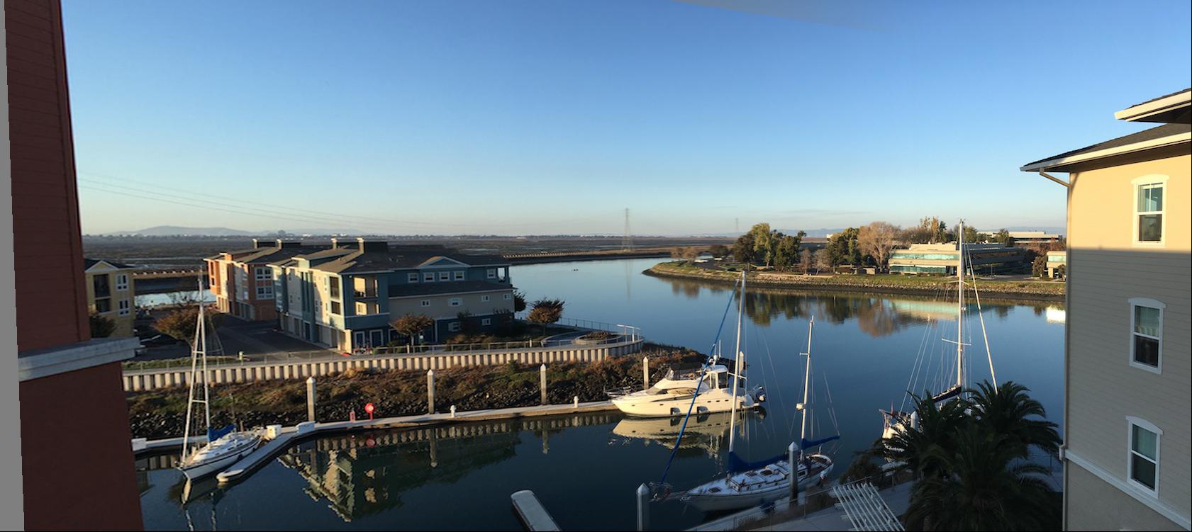
Now that we can recover the homography H and use it to warp an input image, we want to try to create an image mosaic by projecting one image onto the other and blending the overlapping areas to create a "panoramic" image. I will use the following input images to try to create a single long image mosaic:
input 1
input 2
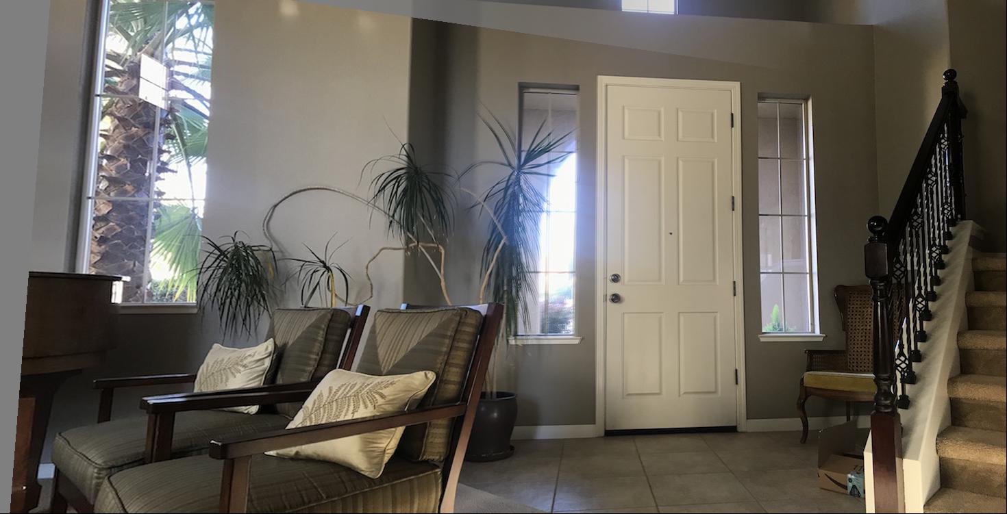
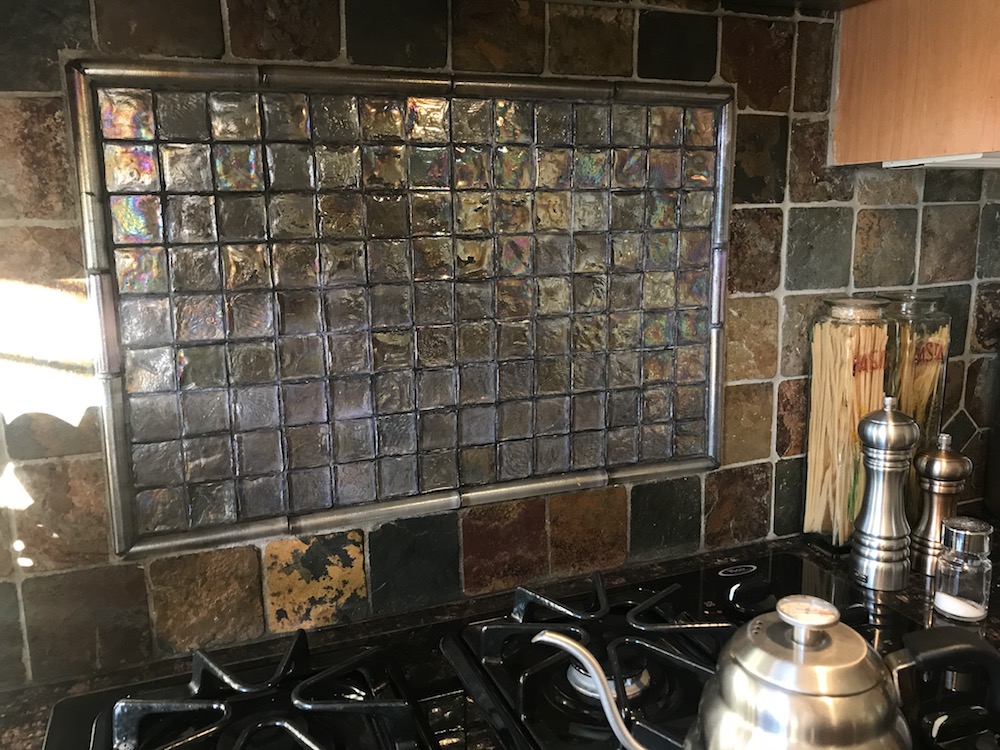
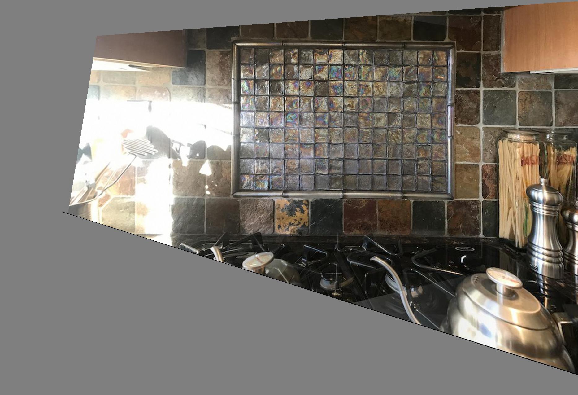
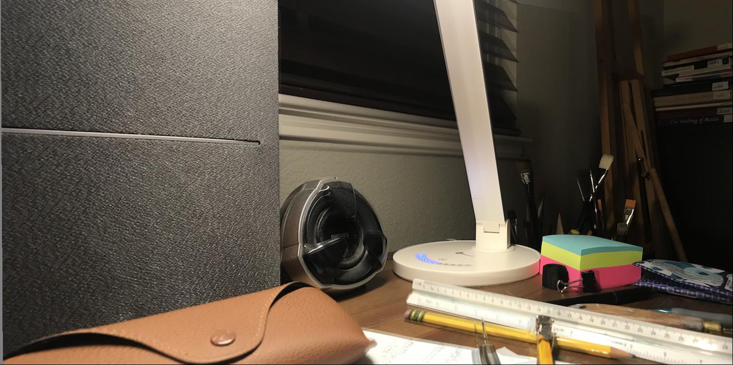
I compute the homography as before between the two input images, warp the first image, and make note of the x-displacement that the homography caused as my shift.
warped input 1
input 2
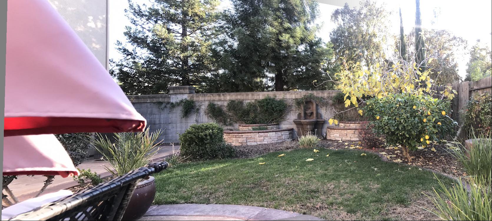
Then, I create a dummy np.zero image of the same height as the two images to combine, but with a width equal to the second image's width plus the shift. Before I overlap the images, I add an alpha channel to each, and in the area of overlap between each image, I drop the alpha off linearly from one image to the other, like a weighted cross-dissolve. I then add the first image in-palce to the dummy image, and the second one with the x-shift, so that the alpha drop-offs overlap perfectly, creating a smooth transition. The result is shown below:

output mosaic
Here are a few more mosaic results:
mosaic
rectified mosaic
Something I thought was really interesting and important about the project is the idea that different viewpoints of a single image can be simulated using a simple projective transformation.
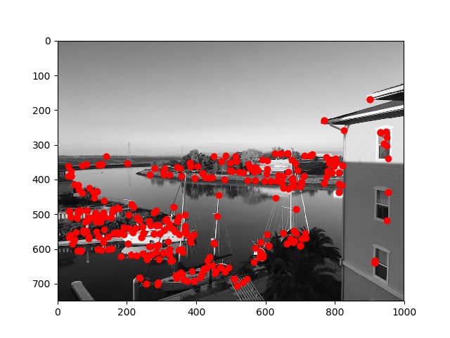
The first step in automatic feature matching is to detect "corner" features, for which we use the Harris Interest Point Detector. The result of the Harris detector on the first two input images I used in the previous part is shown below:
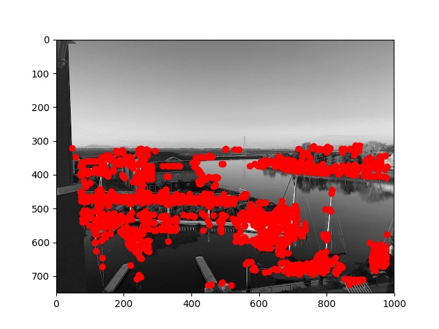

We want to limit the number of interest points used to make automatic feature matching more computationally tractable; and the amount of points detected by the Harris detector shown above is too large. To limit the number of points, we perform Adaptive Non-Maximal Suppression (ANMS) on the set of points coords along with their "corner strength" h obatined by the Harris detector in the above step. We can set a number of interest points n for our ANMS code to find, and take only the n points of greatest "minimum suppression radius" (r_i) defined as follows:
r_i = min(j, |x_i − x_j|), s.t. h(x_i) < 0.9 * h(x_j), x_j in coords
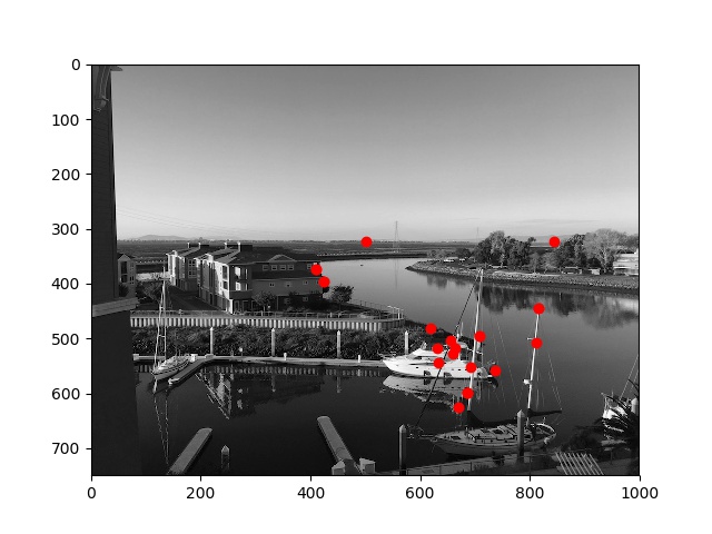
Below are the results of running ANMS with n=500 over the input Harris detected points from the images above:
Harris detected points 1
Harris detected points 2
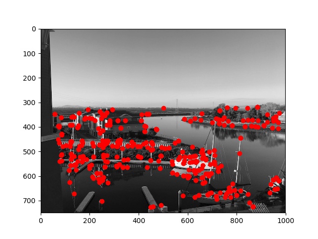
ANMS points 1, n=500
ANMS points 2, n=500
We define descriptors as 8x8 patches surrounding our interest points obtained in the previous step. To mitigate the effects of noise and perspective alteration, we need to blur and subsample our patches. I first apply a Gaussian blur over the image, then take 40x40 samples surrounding each interest point. I lastly subsample an 8x8 grid from the larger patch using a sample distance of 5 pixels, and normalize the subsample so that the mean is 0 and std is 1 (with (a - a.mean)/a.std), and add it to the list of descriptors.
Given lists of feature descriptors over two input images from the previous step, we perform feature matching by computing the SSD between each pair of matches, and consider the first two-NN matches (two lowest SSD matches), SSD1 and SSD2. Then, I take only the matches where SSD1/SSD2 < 0.3.
Below are the points from the previous step, obtained after performing ANMS:
ANMS points 1, n=500
ANMS points 2, n=500
Below are the points that were matched by the method described:
matched points 1
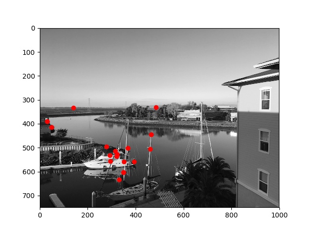
matched points 2
For this step, I implemented the RANSAC algorithm to estimate a homography matrix H over the correspondeces obtained in the previous matching step. We want to further reduce the correspondences we use by only choosing the "best" matches with which to estimate H.
To obtain the "best" matches, we iteratively pick 4 random correspondences from the remaining matched points, and compute a homography H over them. We then compute the error as the SSD between p' and Hp, where p and p' are the points from the 4 random correspondences. If the SSD is below a set threshold (aiming for no more than 1-2 pixels off for each point), then the set of 4 correspondences is added to a final pool of "inlier" points. After about 1000 iterations, a final homography H is computed using least squares over the "inlier" points.
Below are the results of the manually computed homographies from Part A compared with the automatically computed homographies from Part B, using the methods described. The auto-stitched mosaics computed from automatically chosen correspondences look nearly identical to the mosaics from manually chosen correspondences!
manually-computed mosaic
auto-stitched mosaic
manually-computed mosaic
auto-stitched mosaic
In this last one, the auto-stitched mosaic looks even slightly better than the manually-computed one!
manually-computed mosaic
auto-stitched mosaic
One of the most interesting things I learned in this project is how to iteratively obtain better features automatically. Before taking the course, I knew almost nothing about how feature detection worked. From this project (and from project 4), I have obtained a better sense of how images are interpreted by the computer automatically--and that the methods for doing so depend on what you are trying to do with the images (compare facial keypoint detection with the "corner" detection in this project).
Another thing that I enjoyed learning from this project was how to compute homographies over correspondes between images. In general, it was quite interesting learning about the close analogies between linear algebraic concepts like homography and what humans and our cameras "see." It was cool to learn how to enhance our images using the methods implemented in this project.