Part A1: Shooting the Pictures
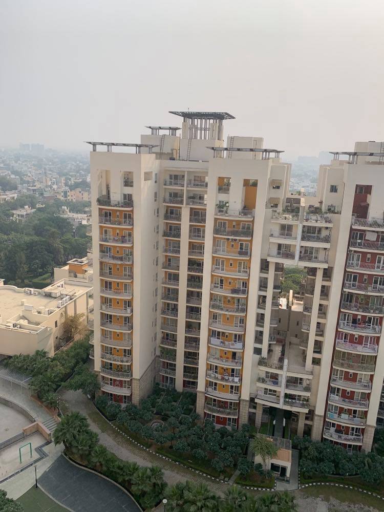
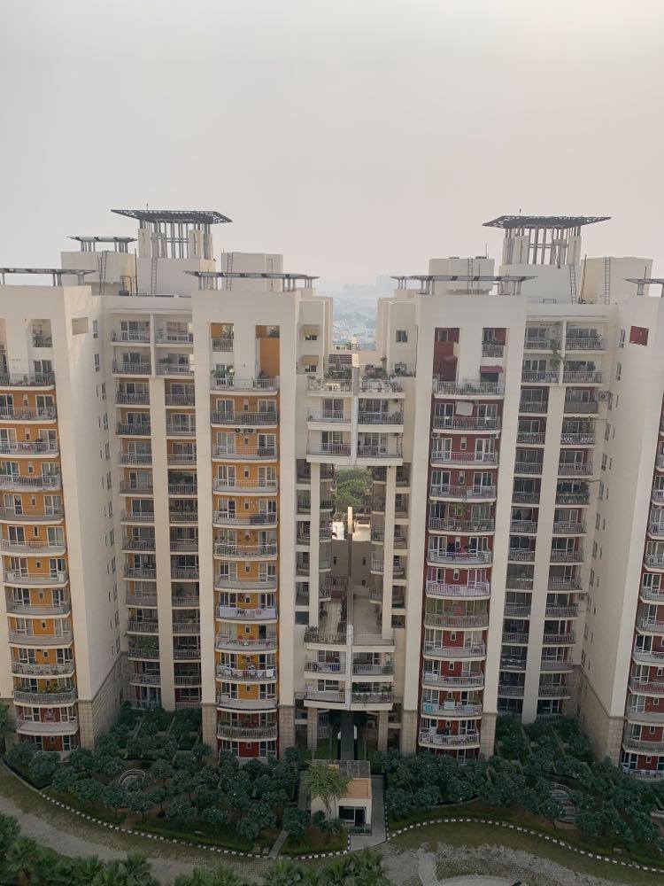
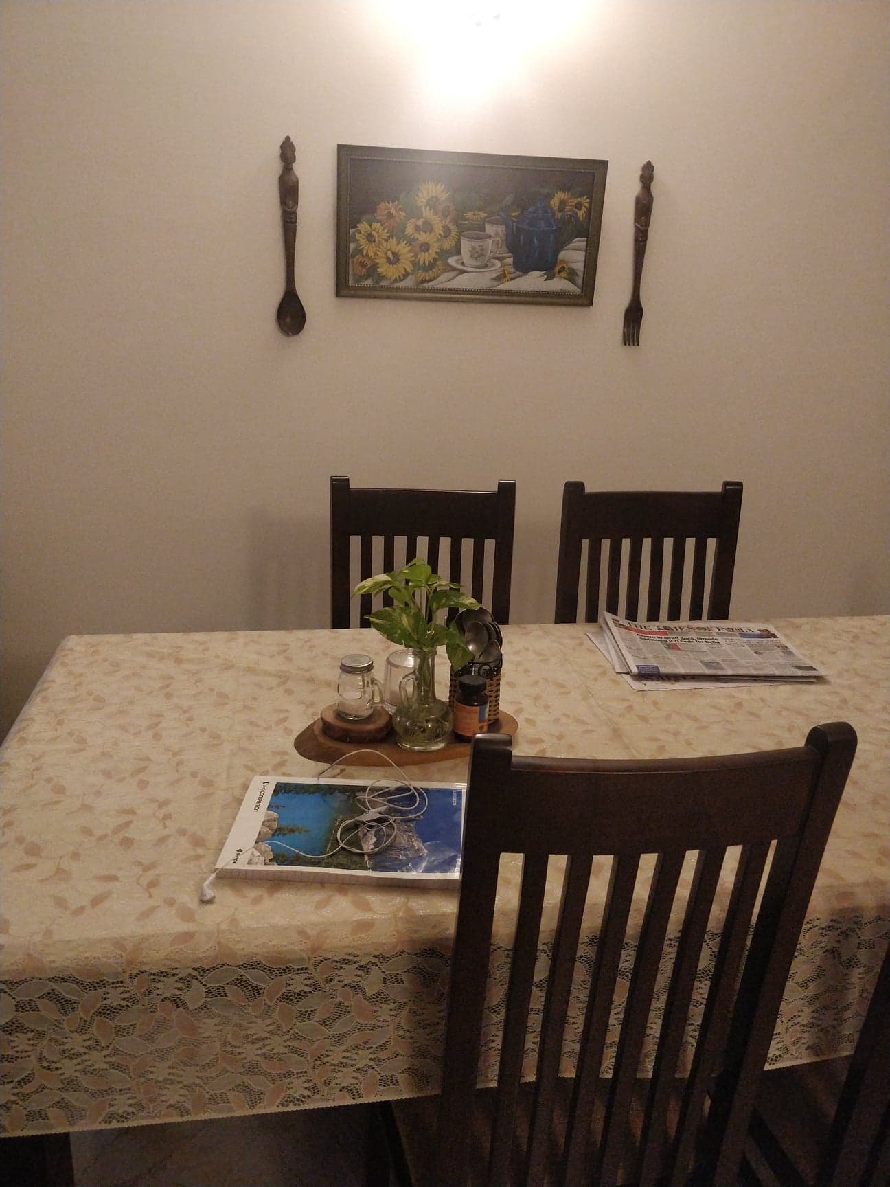
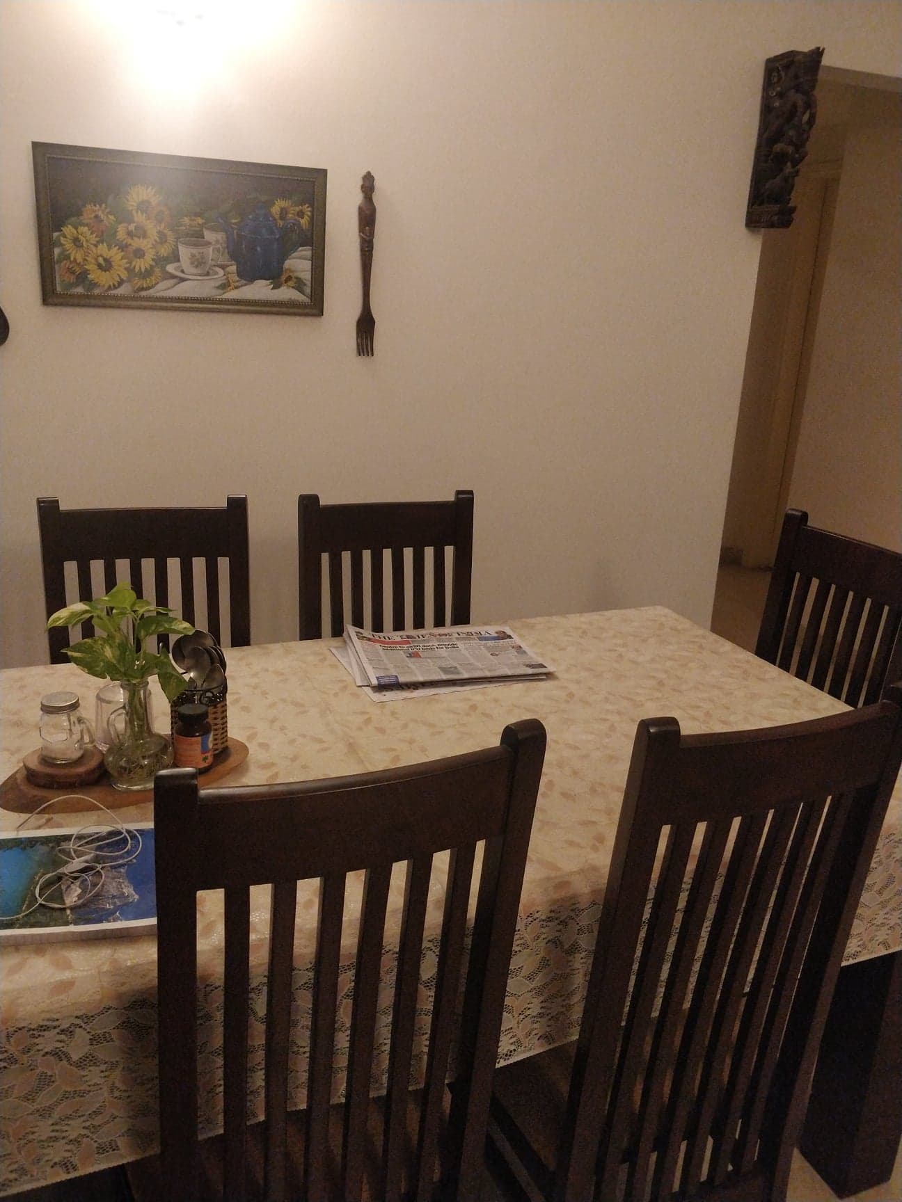
I am restricted to my house because of institutional quarantine in India.Hence I took the following 3 sets of 2 Pictures from my home
Part A2: Recover homographies
I used the Formula discussed in lecture to recover the homography that transformorms a certain point in space in the left image to the corresponding point in the right image. In theory we only need 4 points to get the exact transformation however to account for human error in marking the points I use an overdetermined system with 12 points with least squares used to select the best fitting correspondences to recover the homography. All of this logic is in my computeH function
Part A3: Warping Images
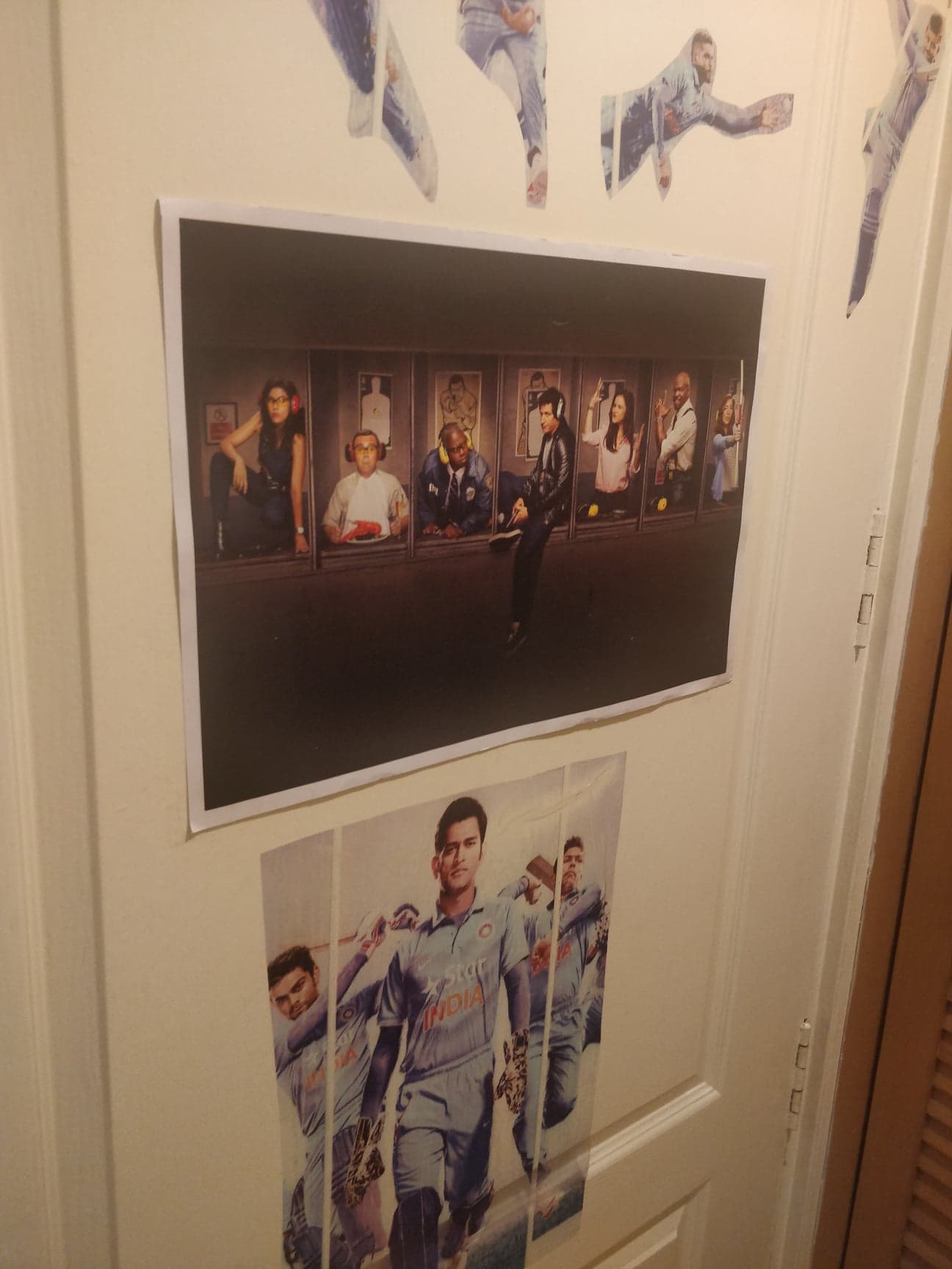
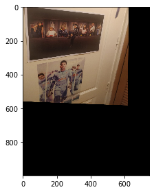
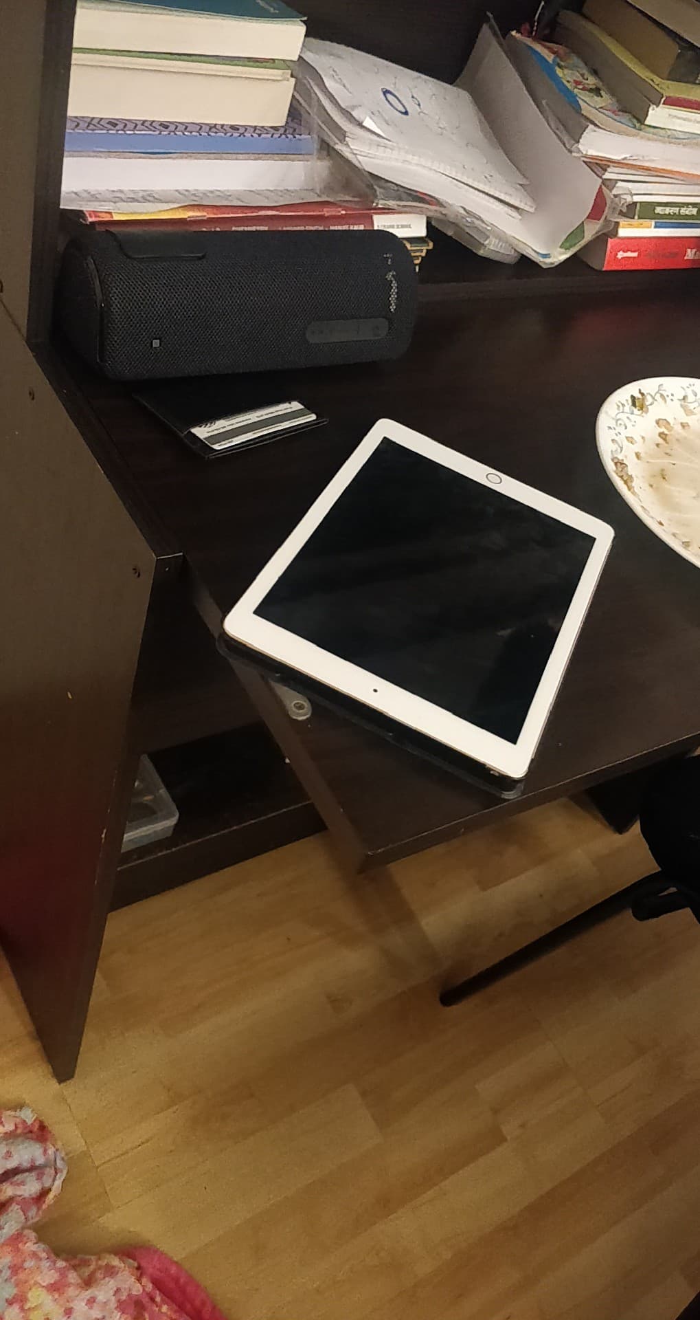
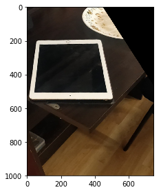
To test out my computeH and warpImage function. I chose one example image as following.
I then assumed that the poster is rectangular and tried to map the first image to 4 points that would form a rectangle to replicate a 'front parallel' view of the poster.
|
|
|
|
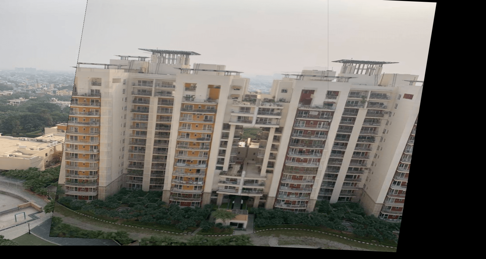
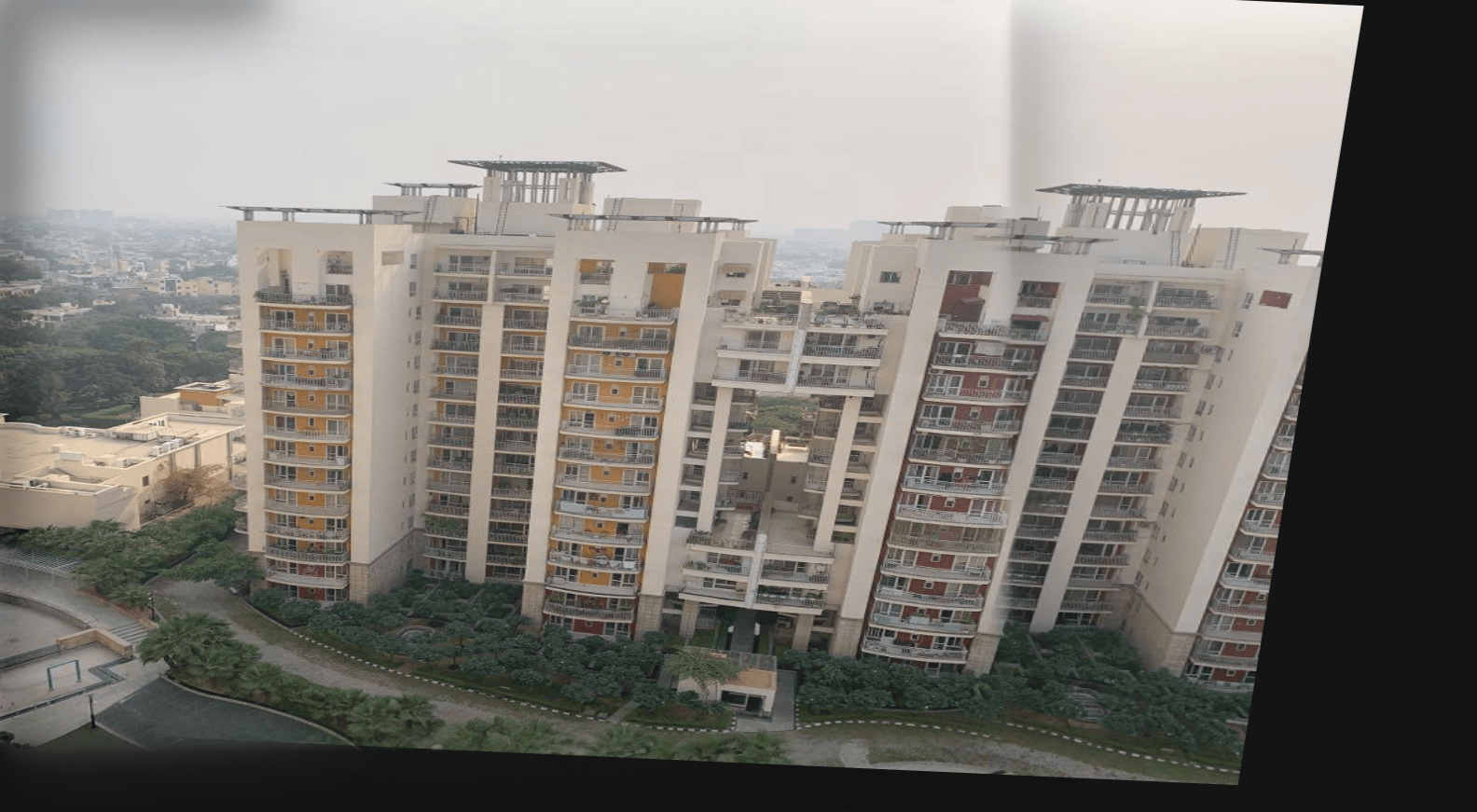
Part A4: Manual Mosaic
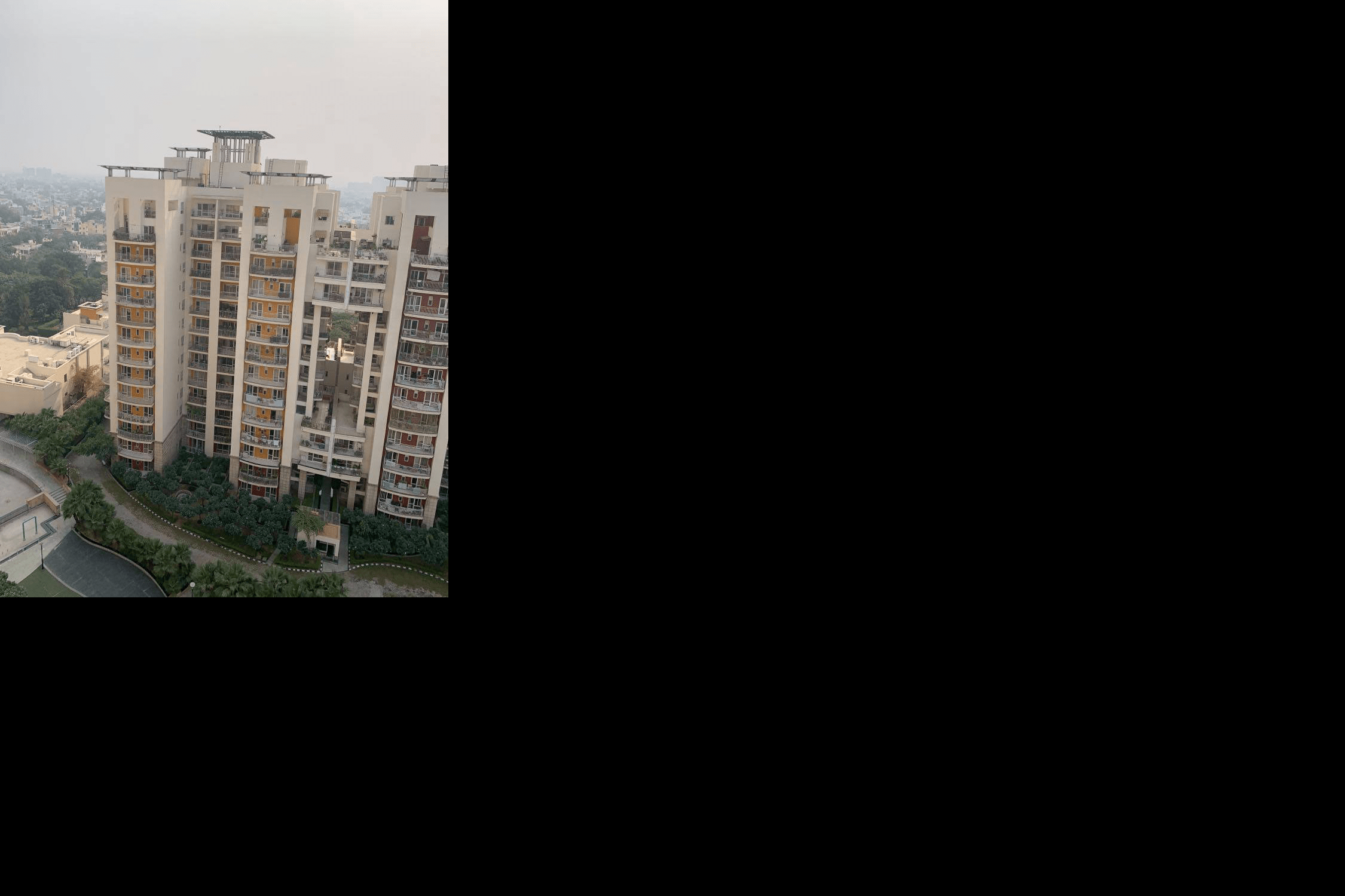
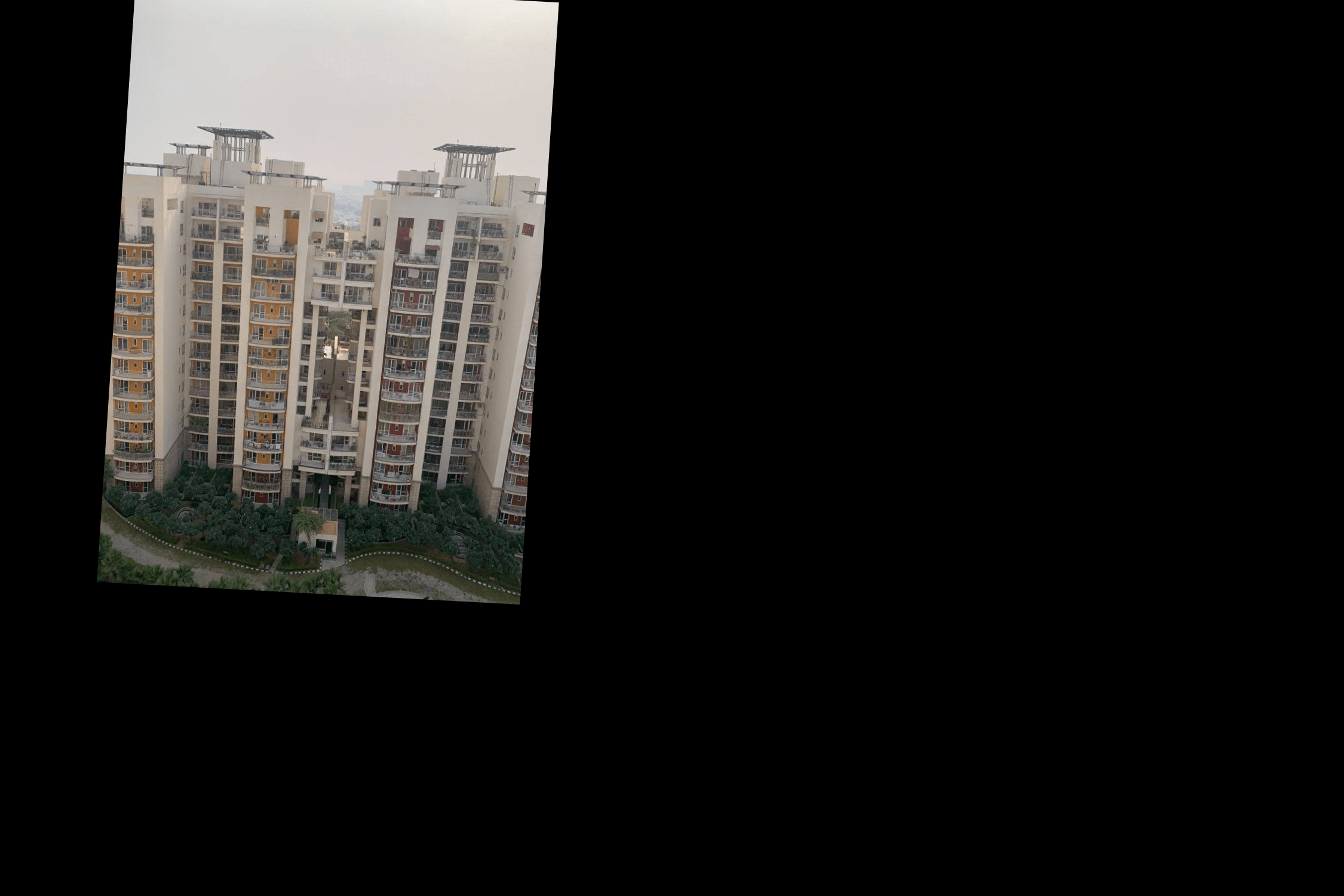
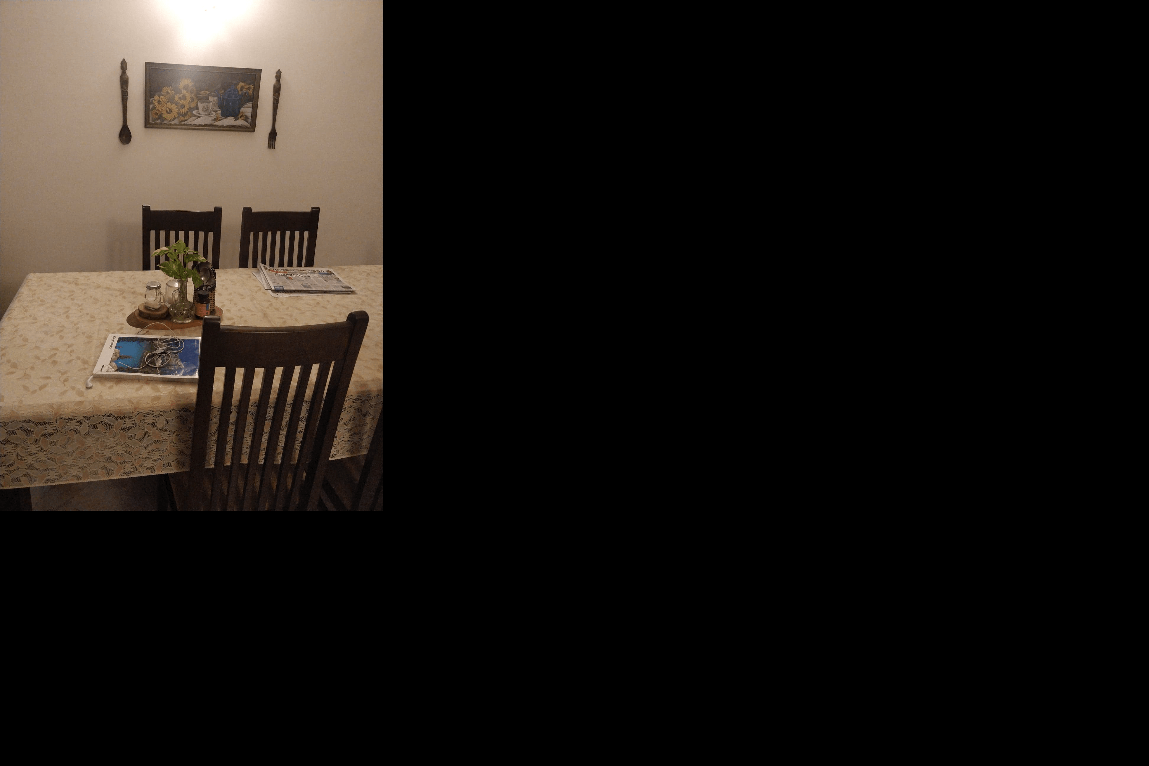
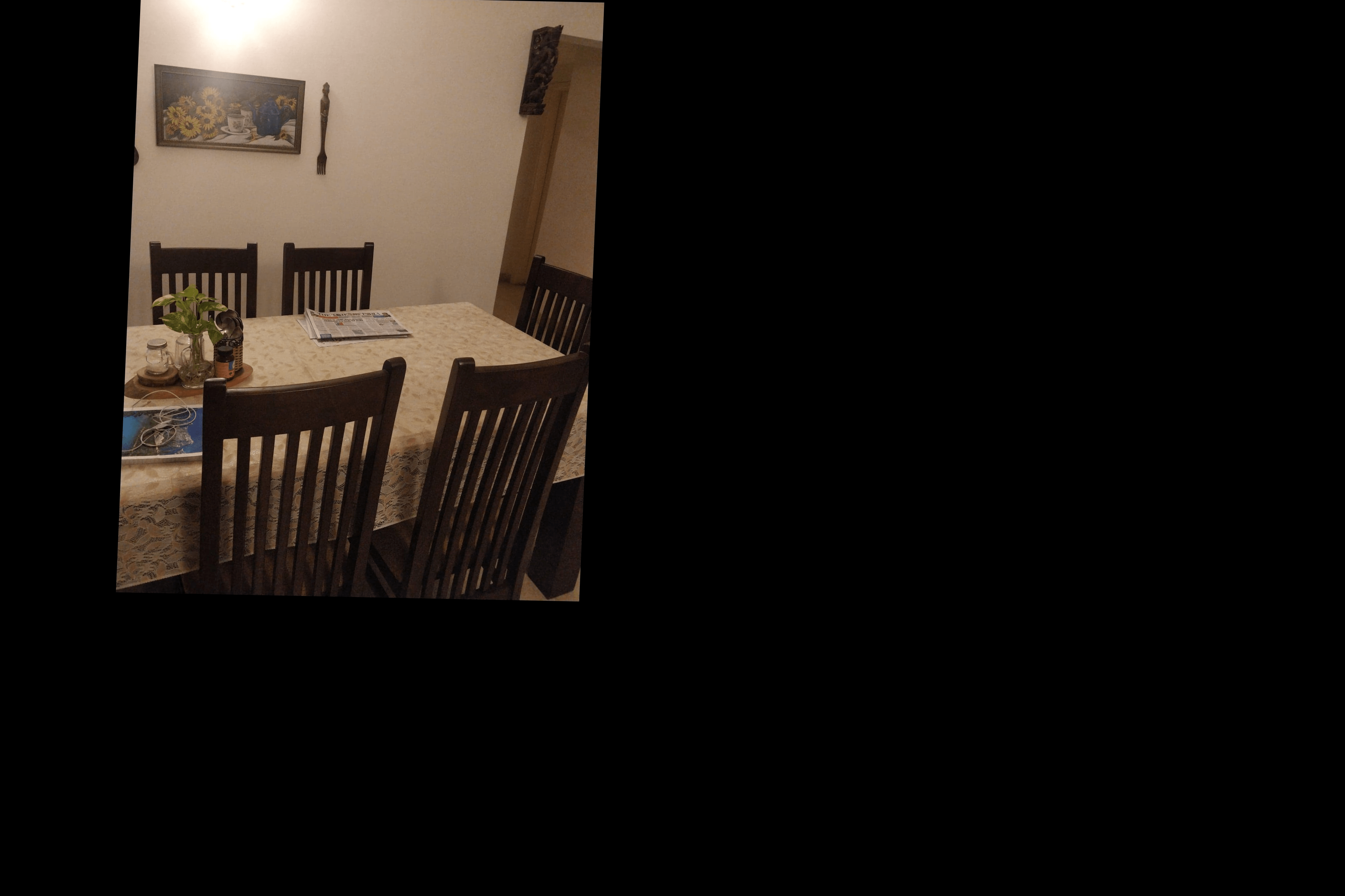
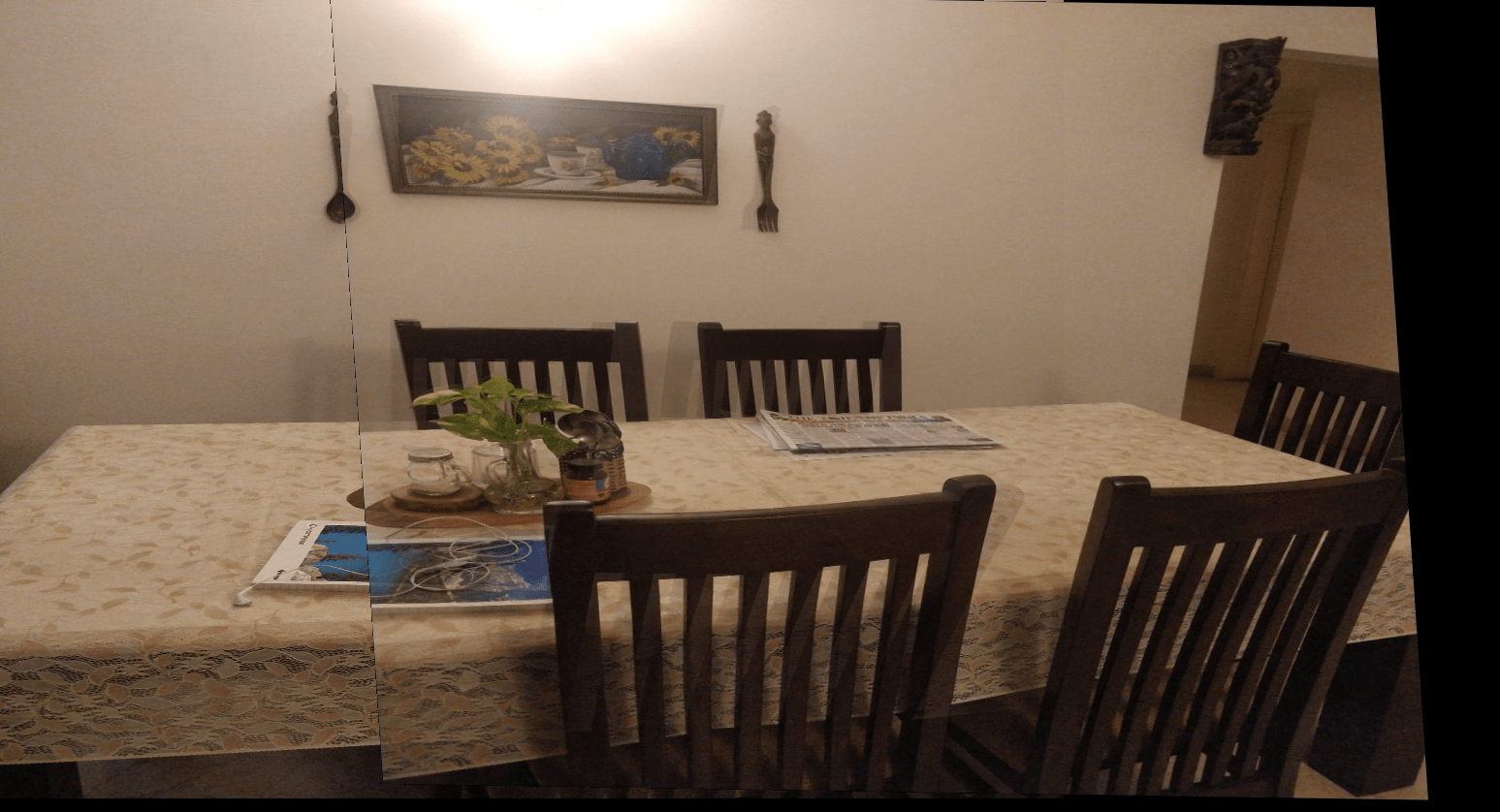
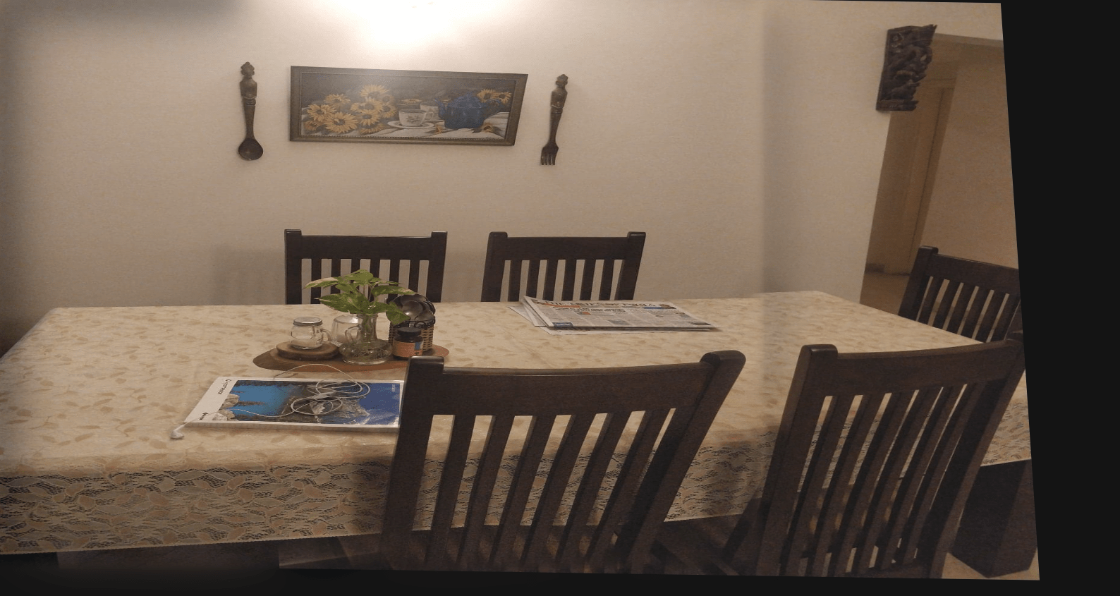
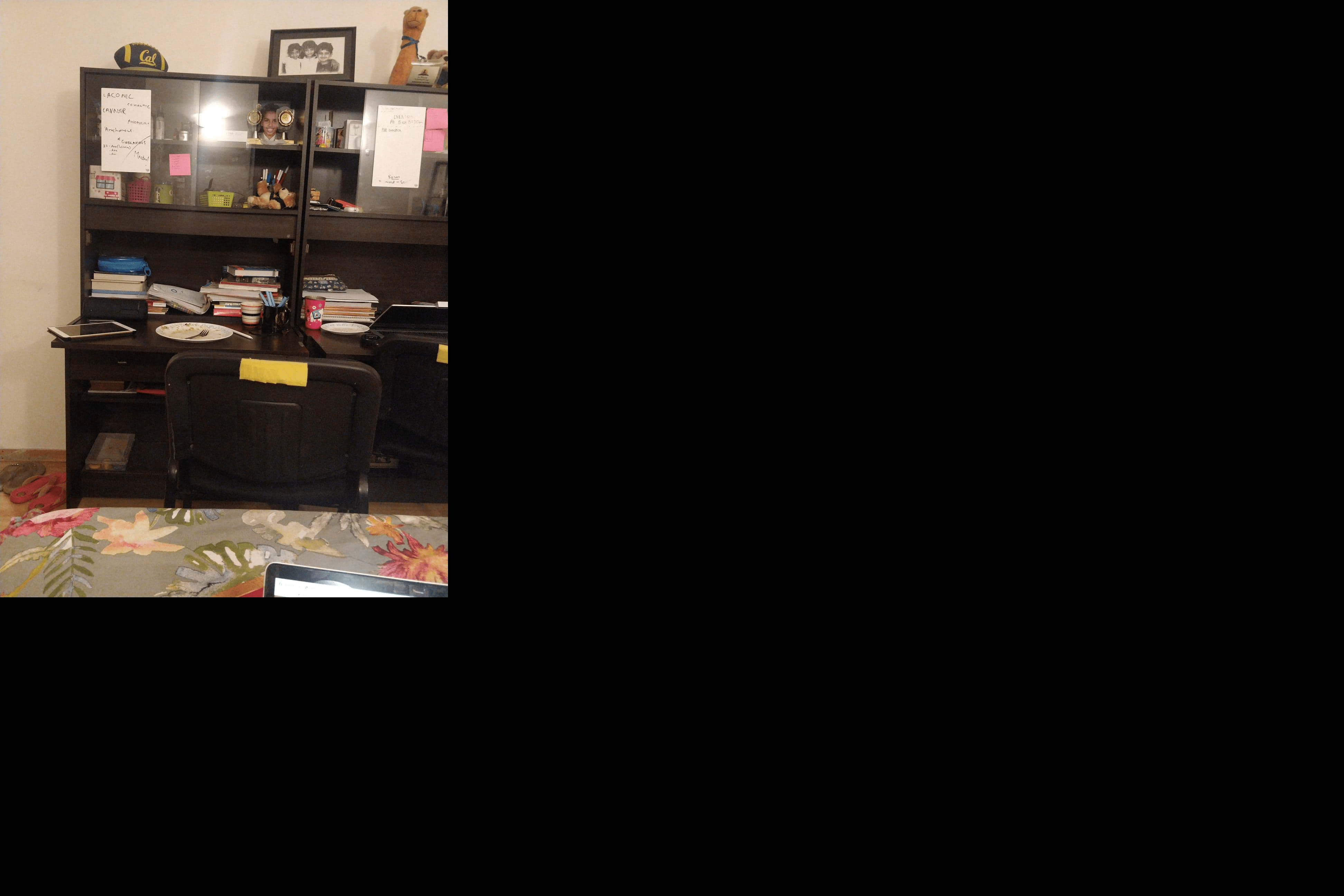
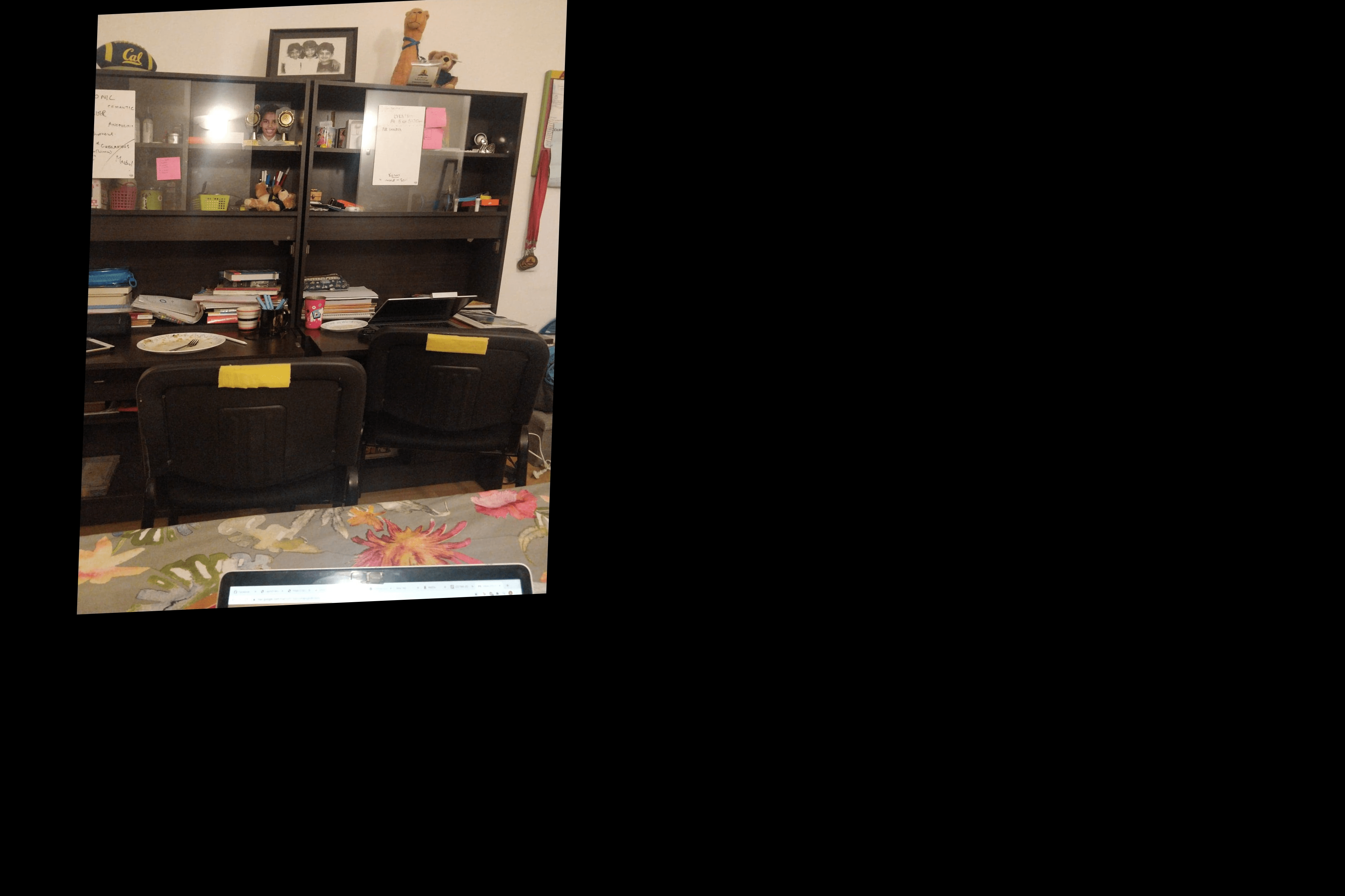
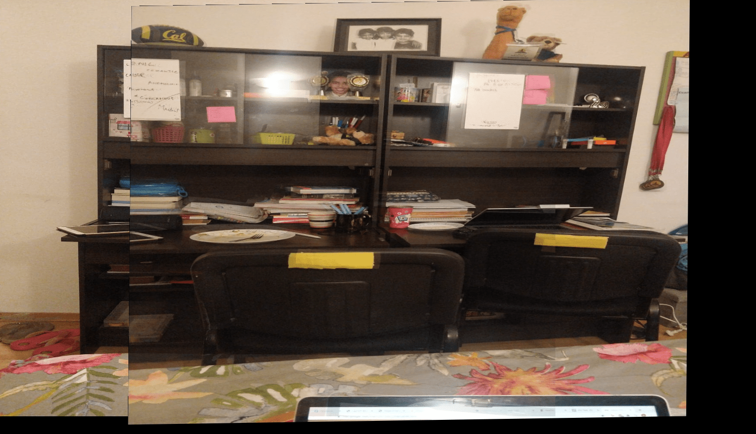
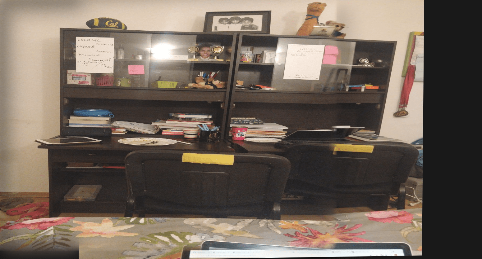
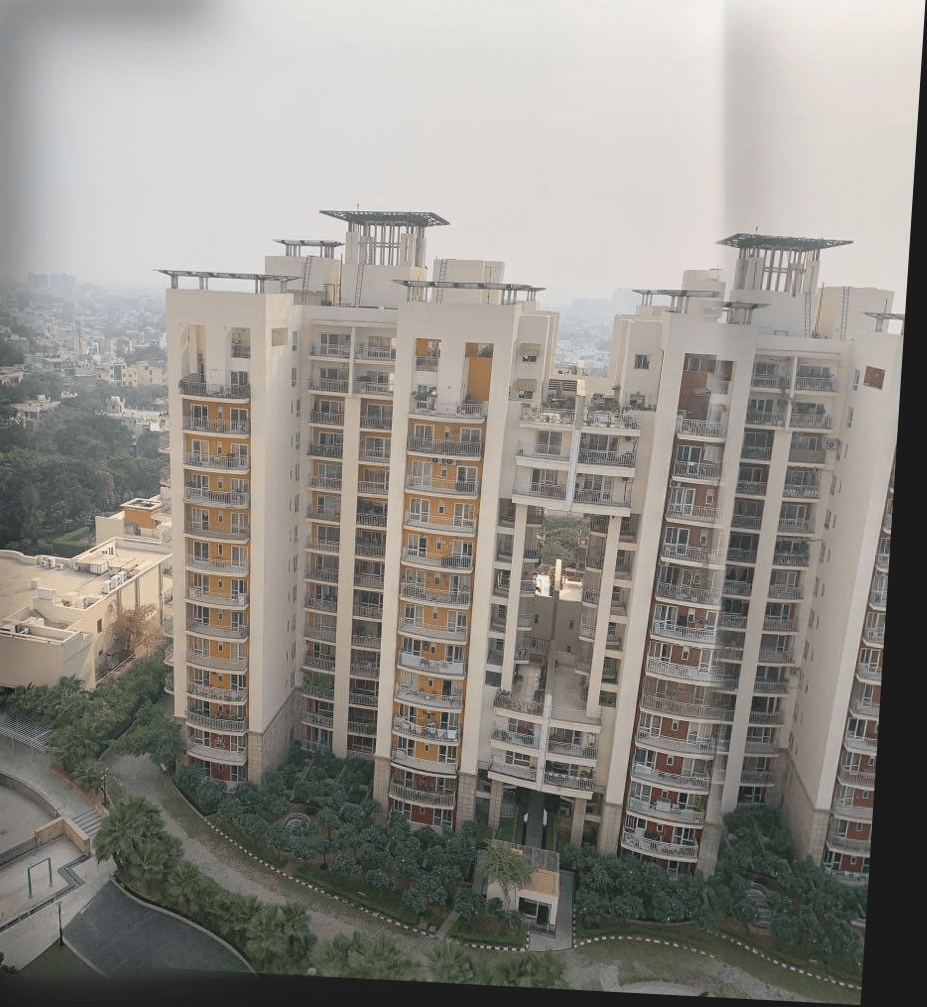
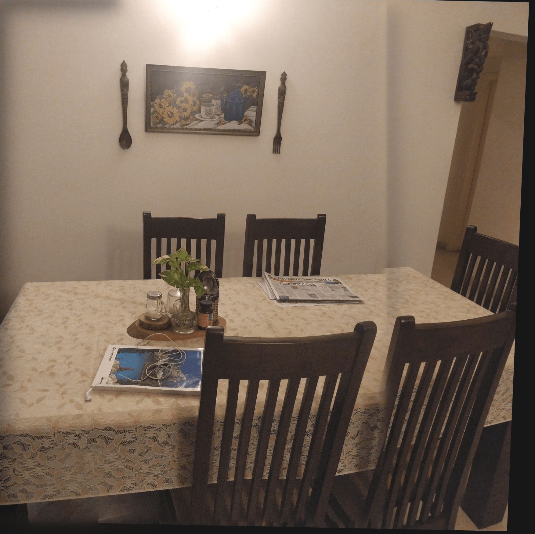
To blend the images- I used both the linear and the lapalacian blend function we used in Project 2 on the result of merging the result of the warped right picture and the stationary left picture(Both images have a considerable level of overlap of about 60% as suggested in the spec) using least squares on 12 manually selected points. The lapalacian results are the las ones on each row and are objectively better than the linear results except in the room case where the high weightage of the first image removes the laptop doscontinuity at the bottom of the picture. Here we have left image, right image,warped left image, warped right image followed by linear blend(0.85 weight of first image) and lapalacian blend(In that order).
Balcony View
|
|
|
|
|
|
|
Dining Room
|
|
|
|
|
|
|
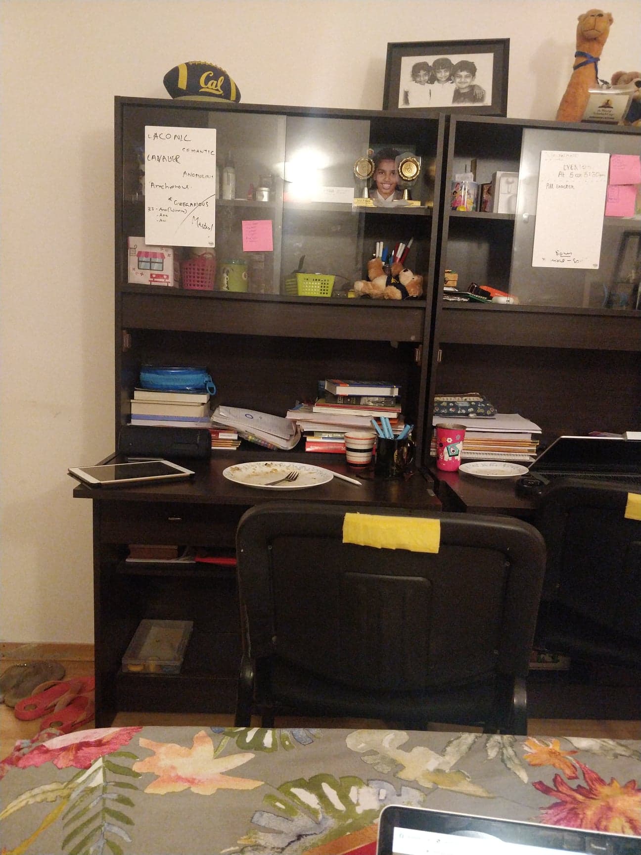
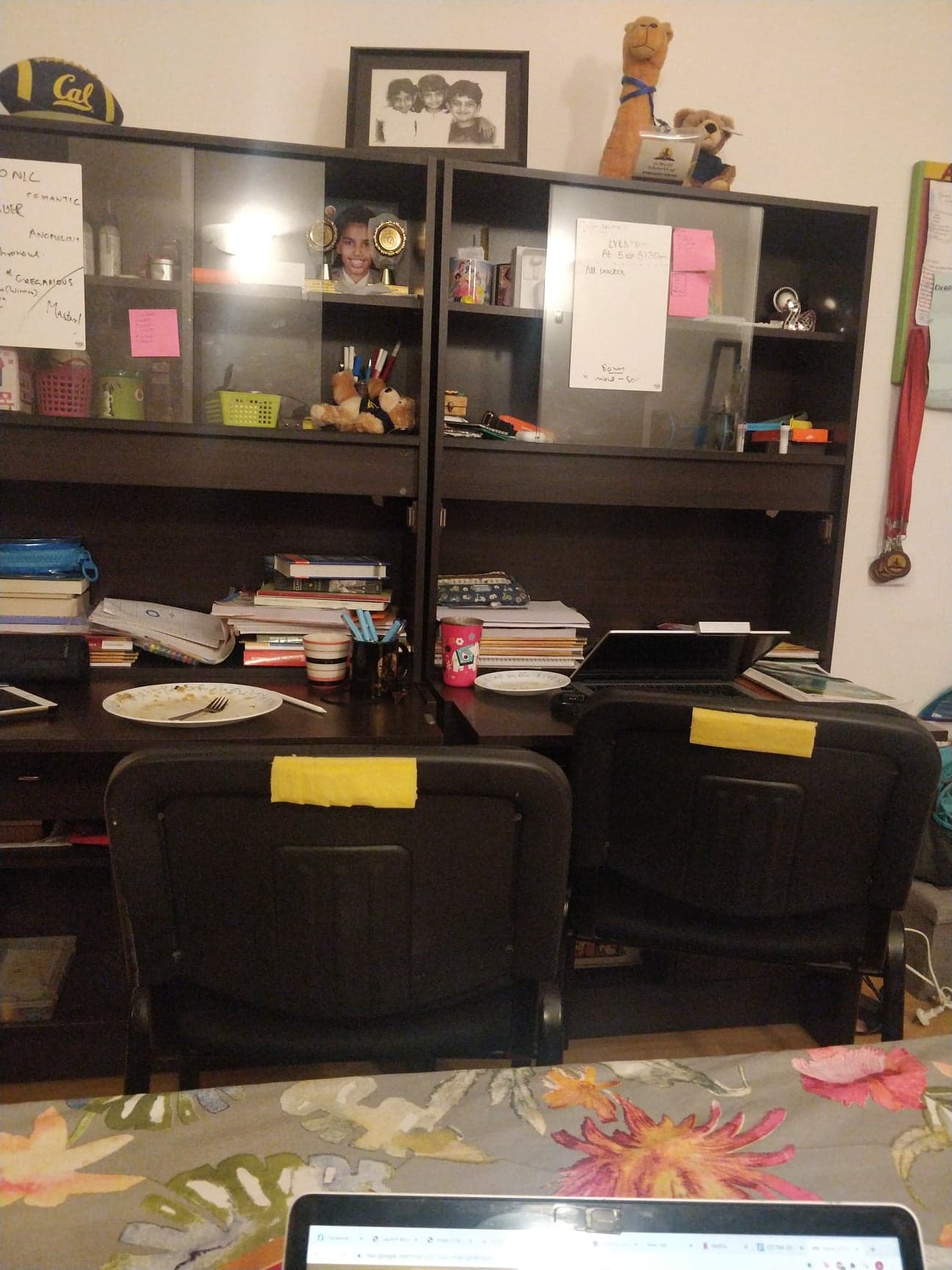
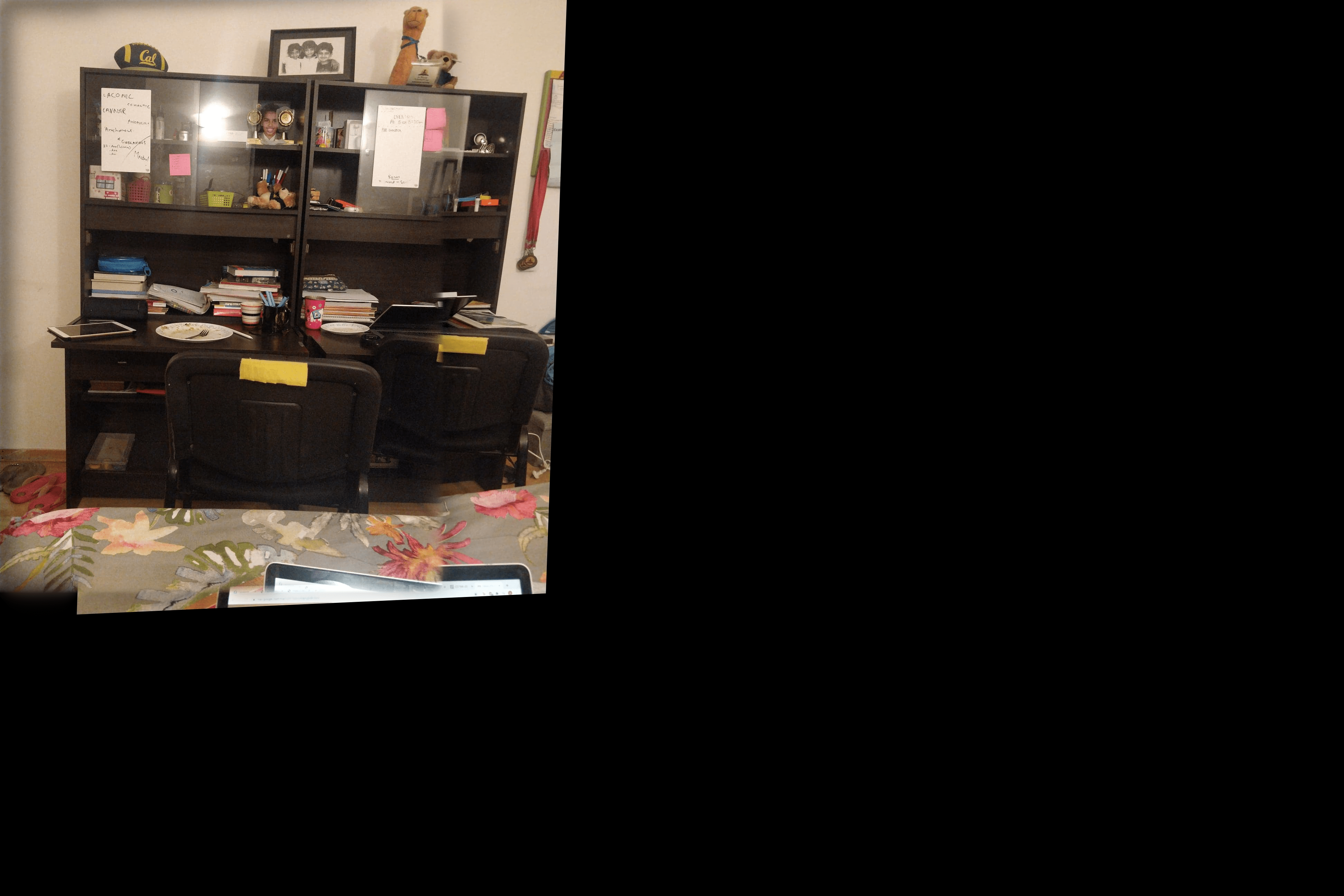
My Room
|
|
|
|
|
|
|
What I've Learned: Part A
I found the concept of basically seeing a second image as if it was taken form the first image's persepctive to be nothing but a homography tranformation that is arrived at by looking at the difference in corresponding points to be very cool
Part B1: Harris Corner Detector
I used the code provided in the spec to detect the Harris Corners of an image. This would be the intial pool of correspondence points that we select a subsample of correspondence points from
|
|
|
|
|
|
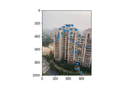
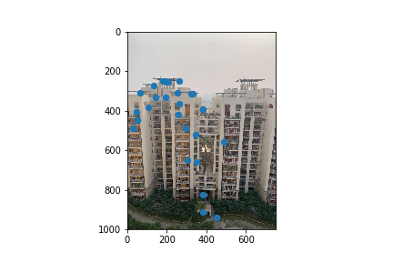
Part B2: Adaptive Non-Maximal Suppression
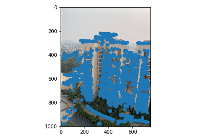
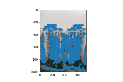
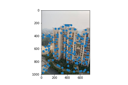
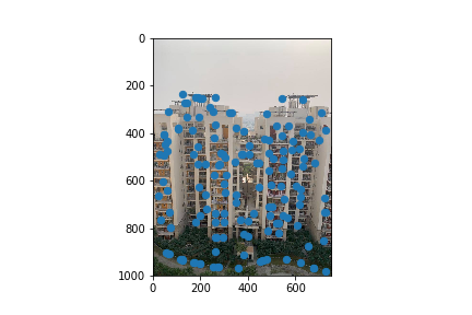
Since there are too many corners, as seen in the last figures, I implemented adaptive non-maximal suppression to choose specific corners that were evenly spaced throughout the image. Now, there are fewer but evenly spaced out corners. I used the 150 corners with the highest radiuses.
|
|
|
|
|
|
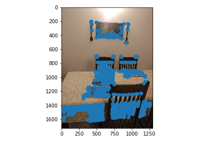
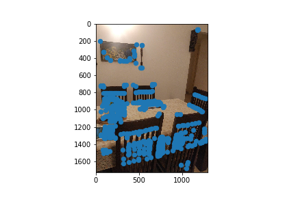
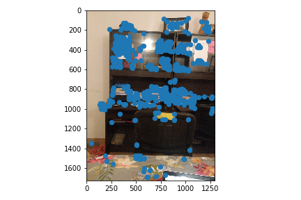
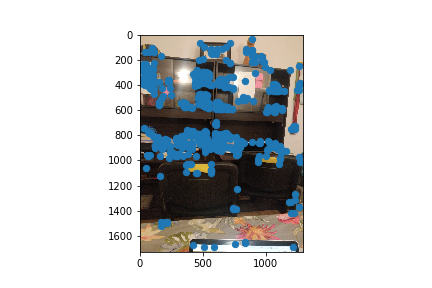
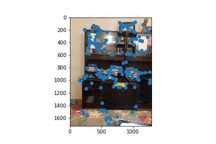
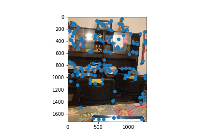
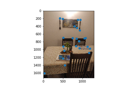
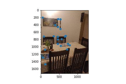
Part B3: Feature Matching
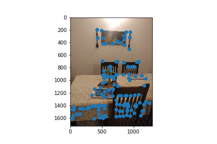
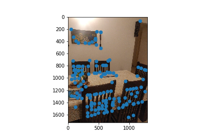
For the next part of the project, I now had to figure out which of these automatically detected corner points corresponded to another harris corner in the second picture and if so which point? To do this I created feature descriptors. My feature descriptor of choice was a 40x40 pixel patches around each ANMS filtered harris corner I then downsized these patches to a 8x8 pixel patch for runtime purposes. I then matched patches from one image to another by finding patches that met my 0.3 1-NN / 2-NN ratio threshold. Here are the subset of my ANMS points that passed this threshold.
|
|
|
|
|
|
|
Part B4: RANSAC
After the feature matching step, I performed RANSAC on the two images corresponding points. This is done to compute a homography that is robust to outliers and involves the following- Choosing 500 random samples of 4 points(From points that have alread been feature mapped to create a homography and find the other points it maps accurately
- Finding how many inliers this computed homography based on 4 random points results in. A feature is considered an inlier if the corresponding matched feature in the other image is less than some epsilon away after applying the 4 point computed homography.
- Use the largest set of these inliers after 500 iterations to compute a least squares approximation of the "best homography" after - This is our chosen homography
Balcony View
|
|
|
|
|
|
Dining Room
|
|
|
|
|
|
Bed Room
|
|
|
|
|
|
As I was restricted by quarantine, I could not take a picture of a landscape which I suspect would have been onteresting to work with Nonetheless autostiching seems to do a marginally better job than manual stitching. This difference is not as big as I would have hoped for however. This might be because of the high number of manual points I selected and the diligence/precision I selected the manual points with. I also didn't play around with a lot of epsilon values and similarity thresholds for ANMS which might have yielded slightly more optimal results.
What I've Learned: Part B
I found learning about the ANMS algorithm to be very cool. The logic of the algorithm seems very ingenious to me and seems to be very effective in increasing the spread of points selected.