The lightfield:

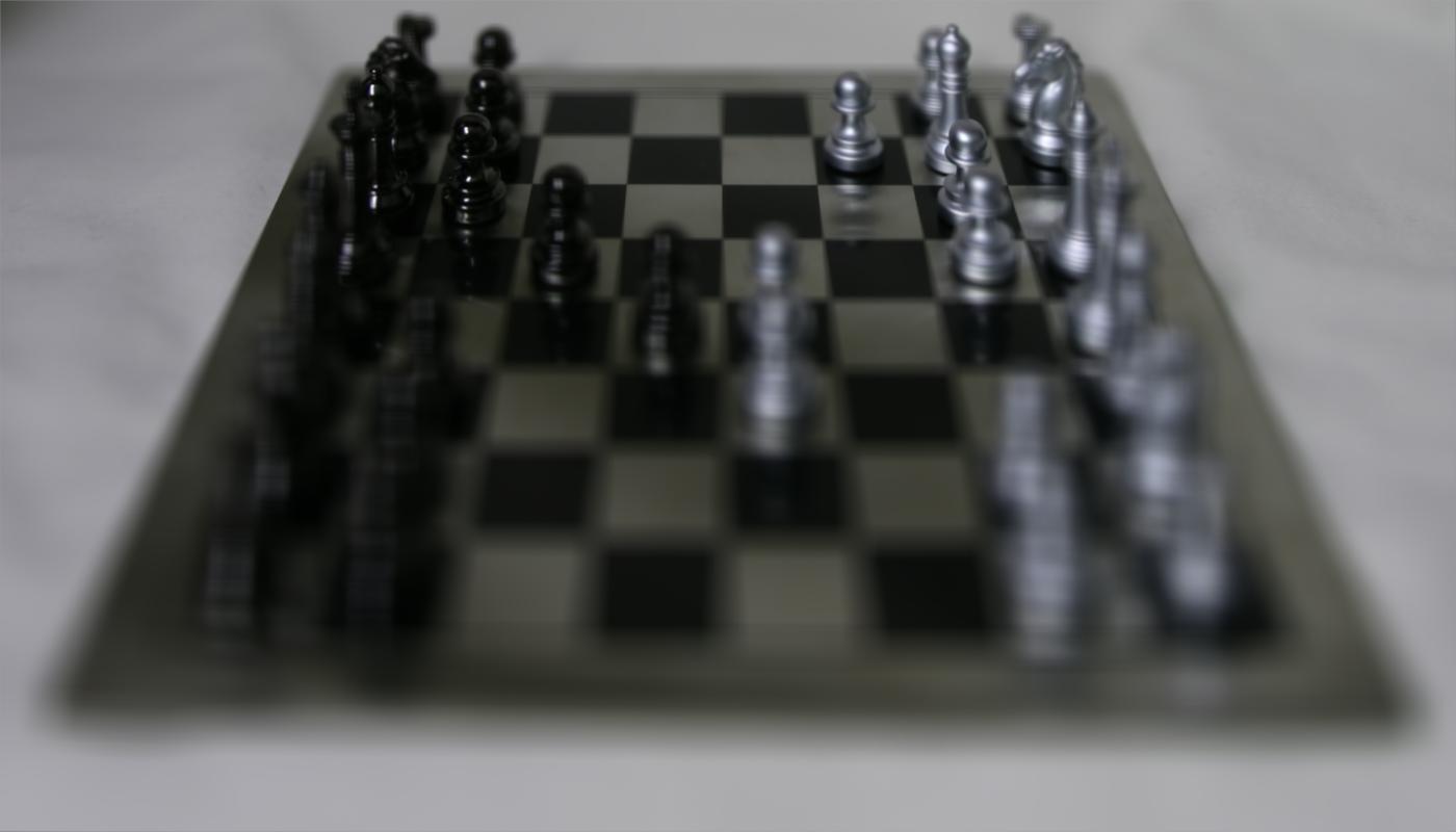
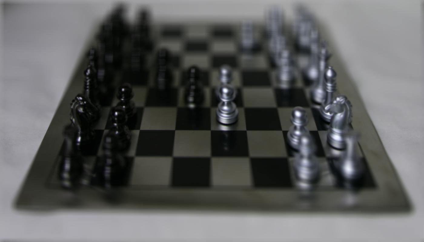
For the first part of the final project, I chose to do the lightfield assignment. The idea of it is that if you take picture of the same scene from several (289!) cameras arranged on a grid, you can not only capture the intesity of light in a scene, but you can also model the direction the rays are traveling in. With this information, you can shift your images to simulate scenes with depth, aperture changes, and refocus to certain points.

Depth refocusing

The cool gif is out of the way, now for how it works: I followed the guide on the relationship between uv coordinates and depth maps from Stanford's website and was able to get decent results. I was stuck for a while trying to solve for alpha, but when I realized we're free to change it to what we like and that it's responsible for doing the shifting, I had a better time with it. I noticed something interesting about alpha-- small, positive values tend to keep the focus far away and larger values have the focus closer to the viewer. I thought about how shifts work in MATLAB and parallax and realized what was happening. I tried negative alphas but didn't get any interesting results from that. I wonder if it would do something else, because the amount shifted really is in the magnitude of the alphas, and the sign would just be the direction the images are shifted in.

Some more detailed results:

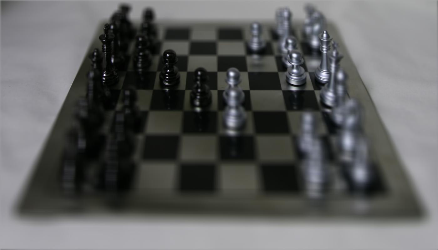
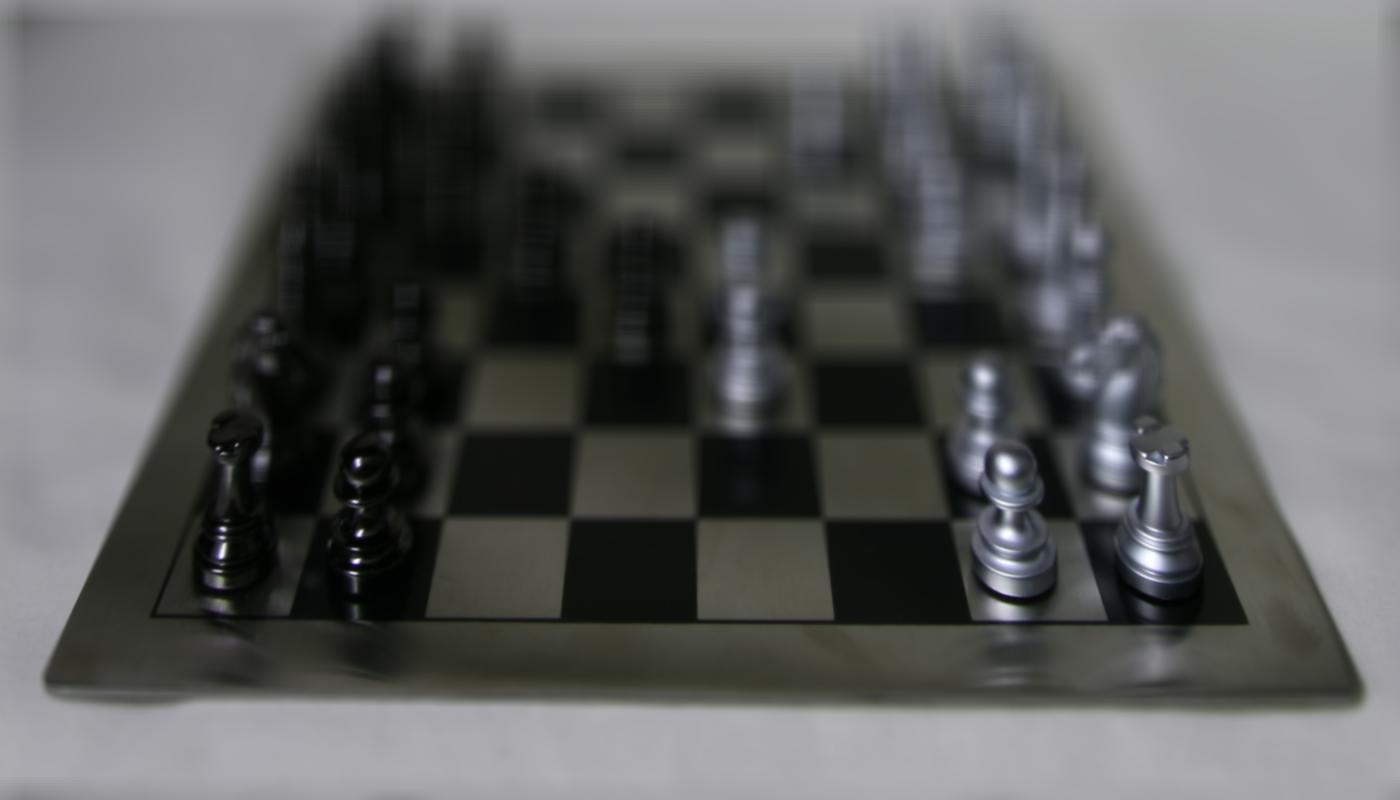
Aperture adjustments

First, a cool gif:

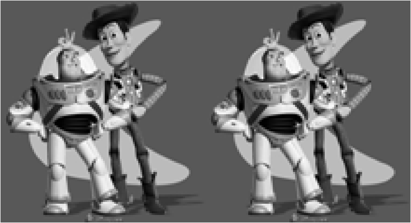
Now for what I did: I noticed that in the web app, if I checked the box for sample angles, I saw a 17x17 grid of little dots that looked a lot like how a camera array might be arranged. I started to play around with pinhole, full, and medium sized aperture, all the while watching the dots. I noticed that some dots were left out of the final picture when the aperture was smaller, or focused in a different area than larger apertures. I also wondered why there's just one big aperture for the camera array, and then it occured to me-- this is the main lens of the camera array, and we choose the width of its opening and that's what determines which rays get in and land on a given sensor in the camera array. This is why when the aperture is small, the entire scene is in focus-- very few rays far from the center (I shifted all images towards the mean u,v) are getting in and only one 'version' of the image is getting seen. When the aperture starts to open up, more images farther from the center are added into the final scene and more 'stories' of how they see the center are coming in. This causes the places where the images disagree to blur more than if you had a pinole opening.

I experimented with the web app for a sanity check and if I set the slider to the middle, these are about the same as what's in the web app.

The 'width' of the aperture means what images were 'allowed' to be summed and averaged. This was determined by distance of the image

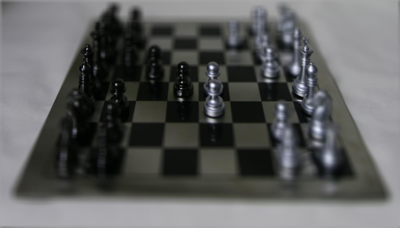
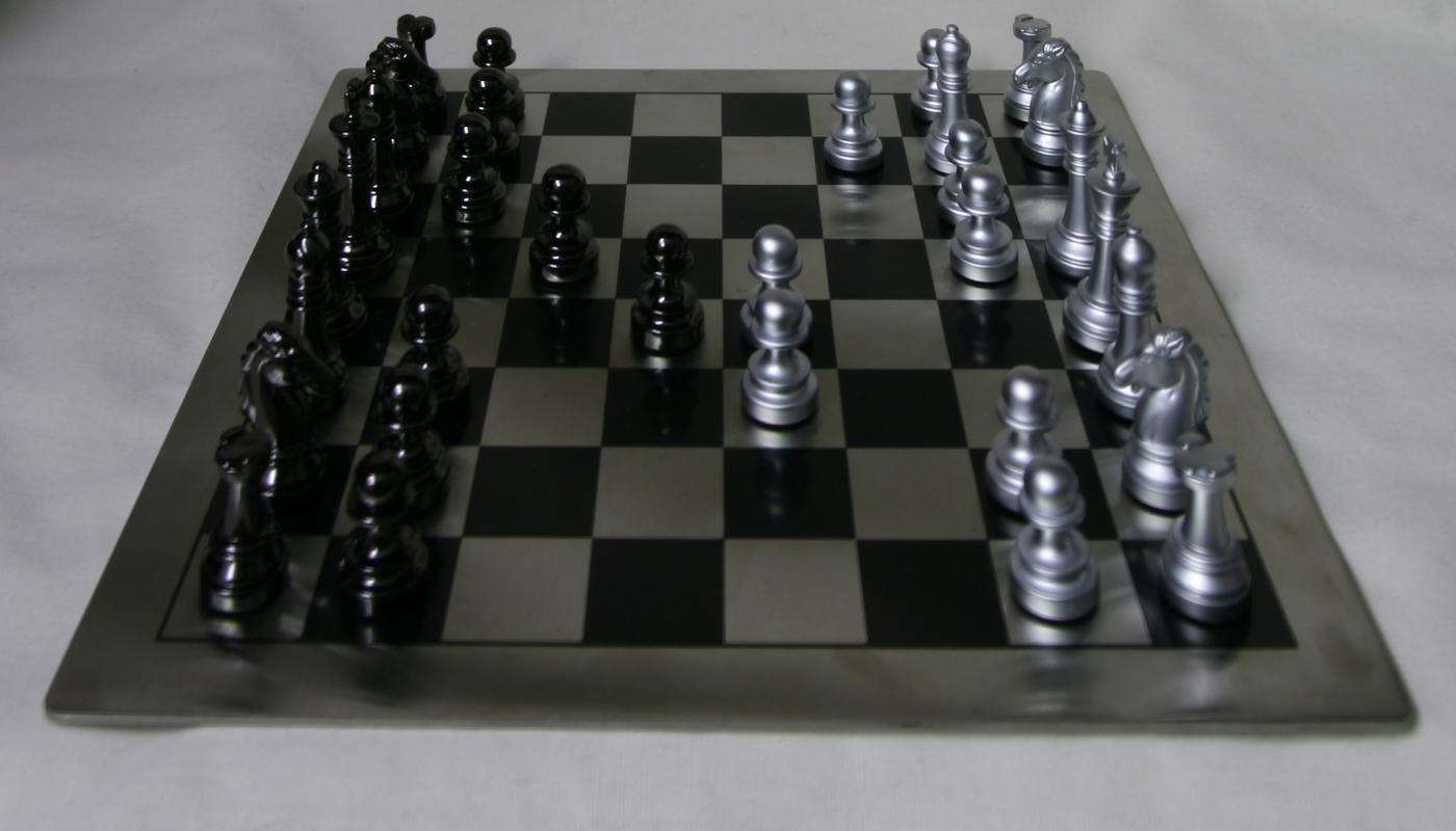
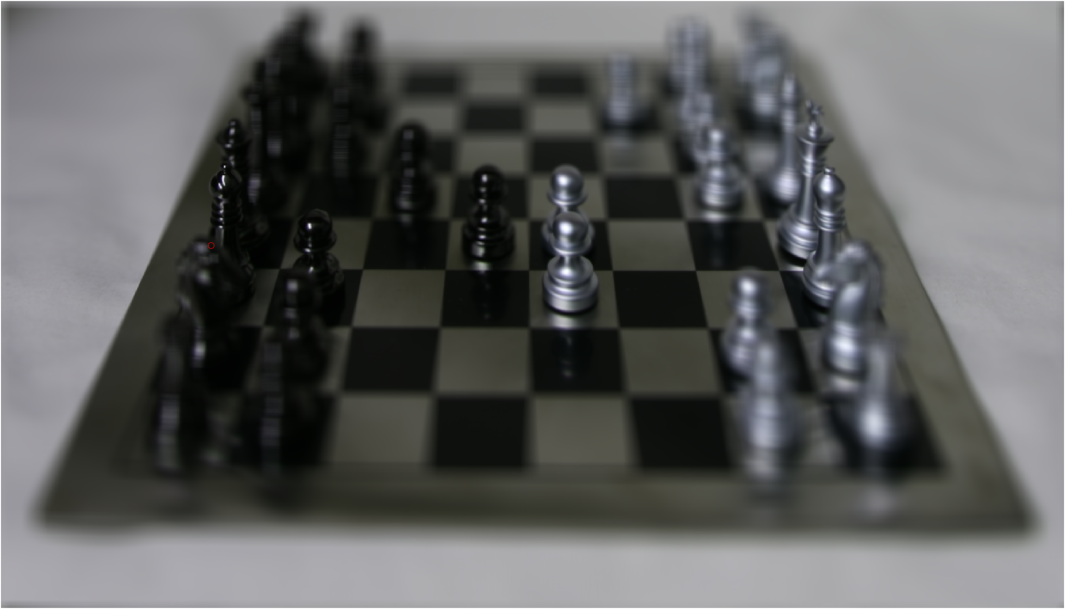
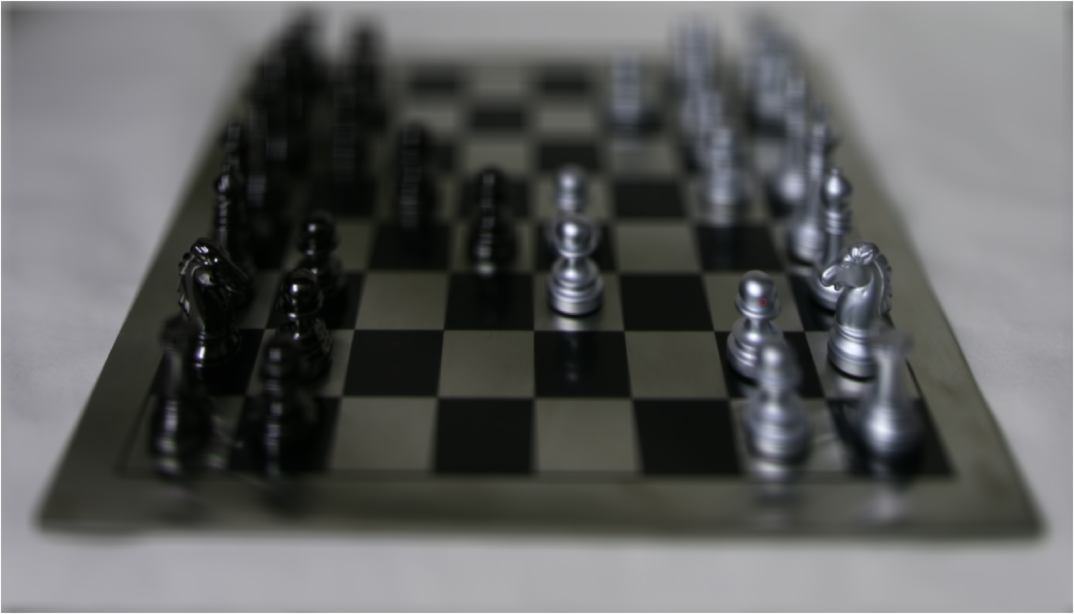
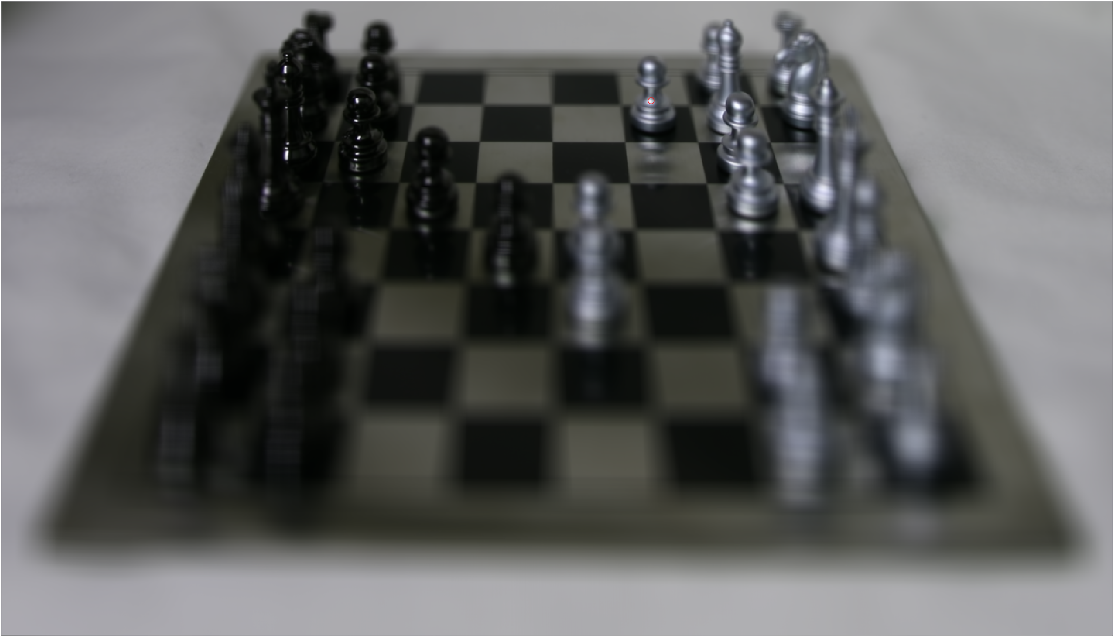
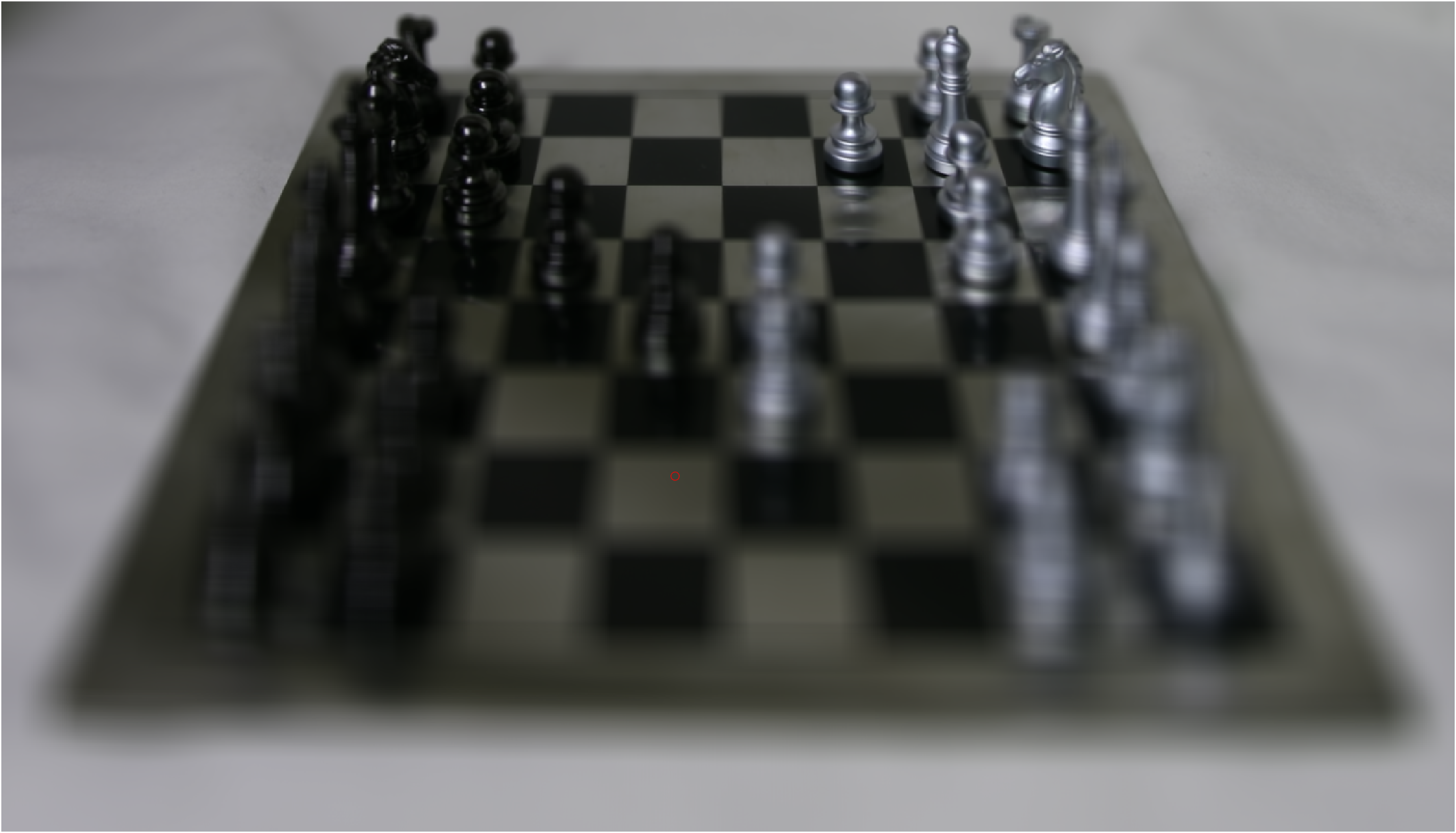
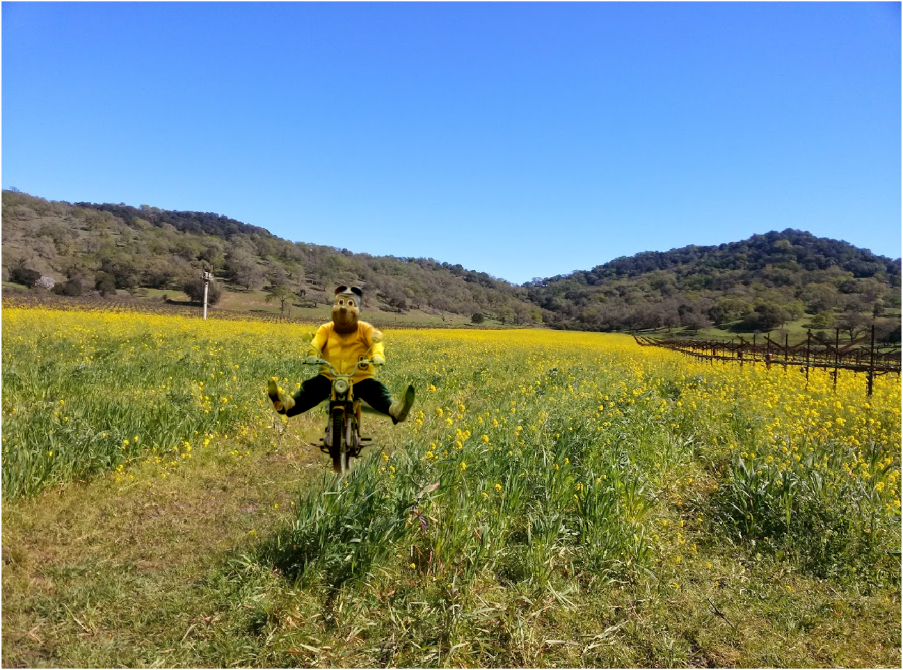
Interactive refocusing

I implemented this part similarly to depth refocusing, except now I have a step where the user can select a point in the image. The shifting window to find similar areas around the point had to be small- it failed horribly if I chose large windows (100ish pixels). I'm not sure why it worked so much better this way, but I wonder if it's because the image is a chessboard and has a lot of repetition within a small space? I'm not completely sure... but after the best shift is chosen using SSD, I solve for the alpha that had to be multiplied to the shifted image's uv coordinates that would have created the x, y this came from. It's pretty much the procedure to create a depth map as linked on the software page, but done in reverse starting from step 3.

What did I learn?

I think it's fascinating how a 3d concept like depth can be encoded in a 2d image through coordinated shifting/average of pictures of the same scene. I also love playing with the alpha values or aperture values to make images that are totally unrealistic or unlike what we would see in real life.

Entering the gradient domain

I did this project because I felt like I had unfinished business with project 2-- I couldn't quite get the mask tool to work the way I wanted, it was a pain to use, and the blends weren't as seamless as I would have liked. With this project and the amount of time we had to work on it, I was able to get deeper into the UI part of MATLAB and was able to get a freehand mask tool that I could click and drag over the to blend image to get a better idea of where things would go instead of just picking a centroid point or bottom point and hoping it would all line up. I think I should have gone farthter into the app editor in matlab to make it even better, but with what I did I feel like it's a good start if I ever come back to it.

Toy example and procedure

In the toy example, we learned how an image can be reconstructed through gradients and matrices. The idea is that if you take the gradient of an entire image then set up a system of equations that reflects the relationship between the points that created those gradients, so like set point a - point b = gradient_ab, but for EVERY point in the image, and a matrix with -1 and ones along the 0th and 1st diagonals, then you can use matrices to solve backwards for the intensities at point a and point b.

Results:

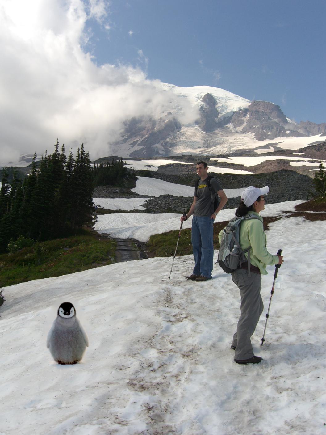
This part is very similar to the toy problem. There are still gradients to find and an image to recreate, but now instead of the whole image, it's a region S defined with a mask tool. I used sparse matrices and 1d indices to establish the relationship between pixels. Since the region S is an extremely irregular, user defined shape that's also 10,000~ish pixels at minimum, regular matrices and bboxes won't cut it. I would have to solve for a ridiculous It might be easier to establish the relationship between pixels since it's all square, but that would require a ridiculous amount of memory and get unnecessarily computationally heavy. (I tried, matlab was not happy making giant matrices 26 GB in size). So I first got the tightest bbox I could around the mask, then made a mask in that bbox of the 'eligible pixels' and made a sparse matrix that was [eligible pixels + 1] rows by [eligible pixels] cols.

Since I had extracted an irregular shape, the pixels didn't have a consistent formula to access their neighbors in the sparse matrix. So what I did was create 4 vectors of 0s and -1s depending on whether the jth pixel in that vector was a neighbor of the pixel in the ith row of the sparse matrix. Then, I assigned those vectors to the -bbox_width, -1, 1, bbox_width diagonal of my sparse matrix, with a vector of 4s along the main diagonal. I created a vector of gradients for all eligible pixels according to the formula in the spec-- even if a neighbor is outside of S, I noticed that no matter what, s will get its gradients calculated, but vj will be a constant. So the vector b was essentially the gradients of all pixels in s for all 4 of their neighbors. Then, I index into all the pixels that had a neighbor outside of S and added the value of the pixel at j in image t to the gradient so that when I solve for vi, that -tj will already be factored into the bi that I set it equal to.

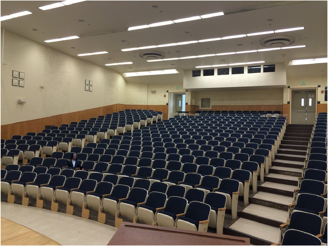
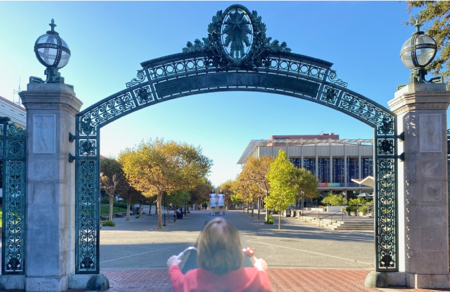
Results for regular blending:

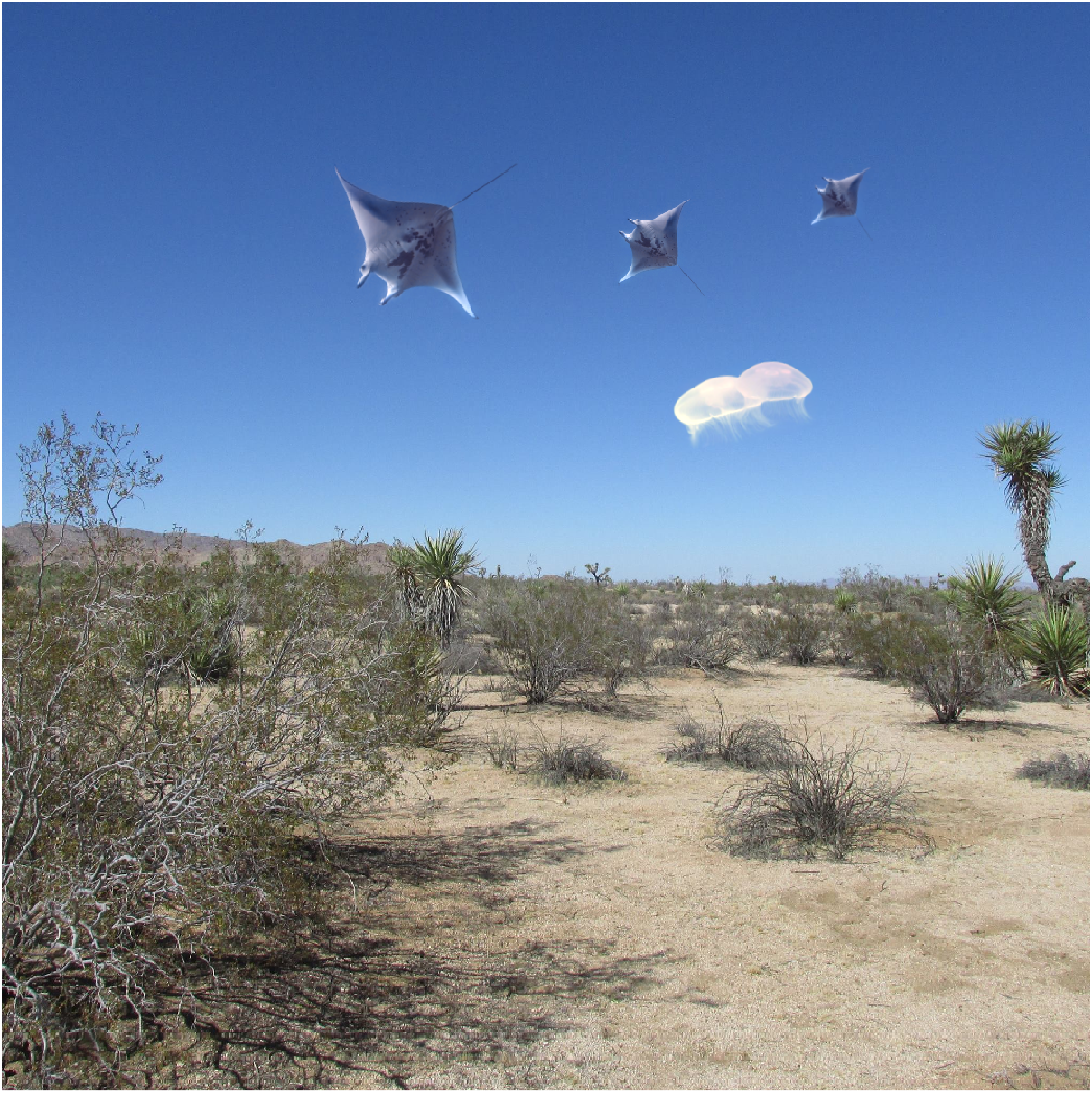
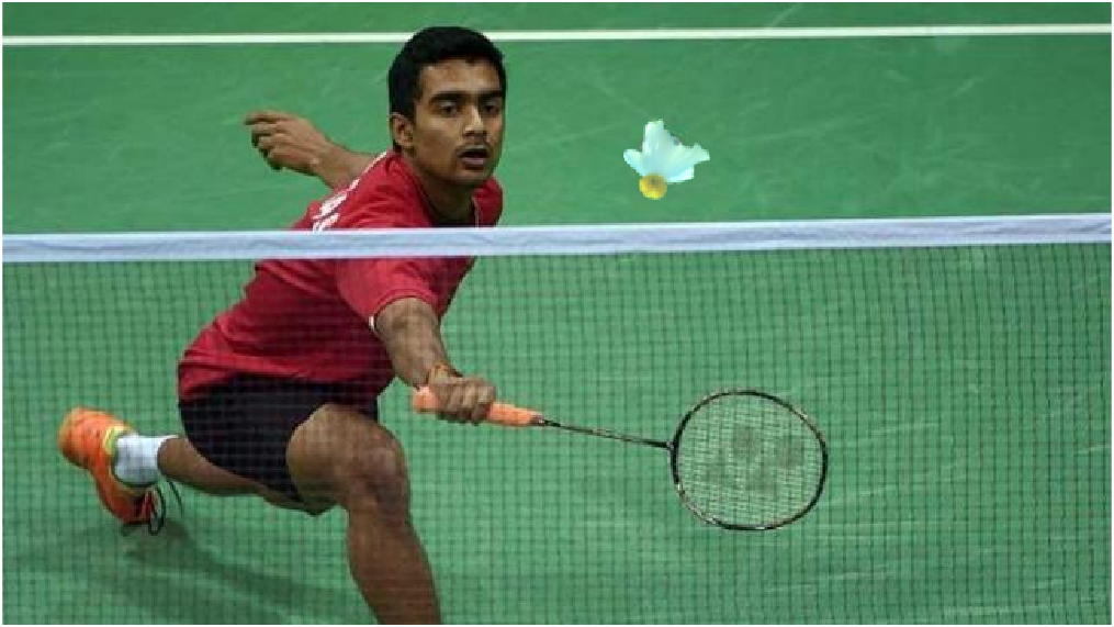
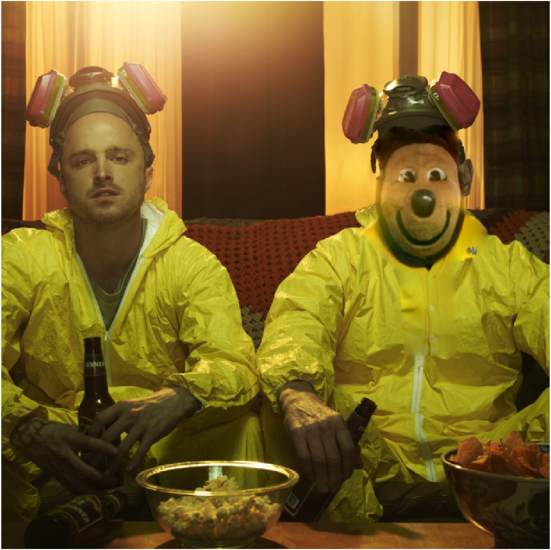
I also implemented mixed gradients by doing a check to see whether a gradient in the source image had a greater magnitude than one in the destination image. Whichever was larger took the place of the s in the original equation. I noticed that this worked very well if I wanted the object to blend to be a little transparent or not completely take over a portion of the image. This produced some interesting results, although I don't think I really captured 'realistic' blends with either technique.