
For my final projects, I've chosen to do Gradient Domain Fusion and Light-Field Cameras. In the first project, we use Poisson blending to combine objects from different images and create interesting results. In the second project, we make use of data from light-field cameras to perform digital refocusing and adjust aperture size.
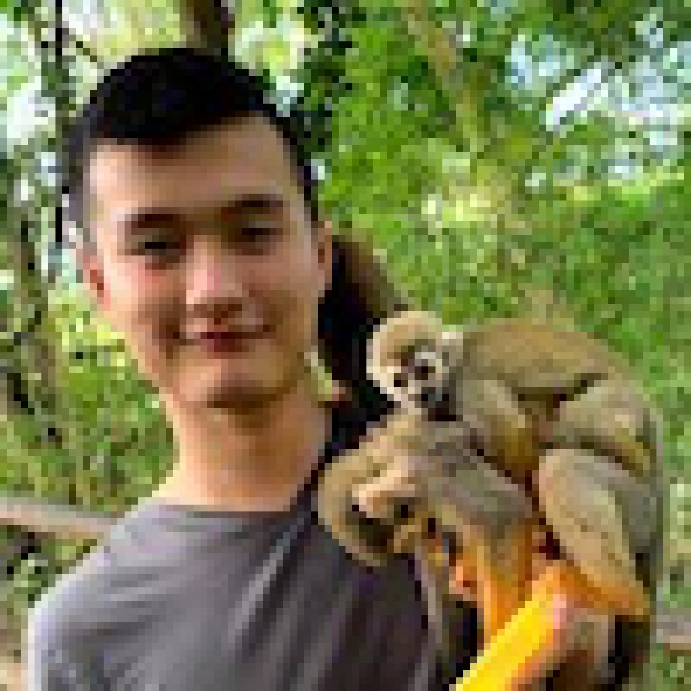
One way that we have learned for blending images is multi-resolution blending using Laplacian pyramids. However, another way that may work better sometimes is Poisson blending, which focuses not on the overall intensity of an image but the gradients, which is what our eyes care about most in identifying objects. Before we get to Poisson blending, we first complete a toy problem to get some practice on the computation involved. Below, we attempt to reconstruct an input image using linear least squares by setting up linear constraints such that the final image's vertical and horizontal gradients match the original image as closely as possible. Additionally, we require that the top-left pixel has the same intensity as the original. With just these constraints, we are able to perfectly reconstruct the original image. In my code, I defined a function toy_solve that takes in the source image as a parameter and outputs an image of the same size and appearance.
| Example Name | Original | Reconstructed |
|---|---|---|
| Me (Leon) | |
|
Now that we've built up some intuition on how to solve this kind of problem, we can tackle the actual goal of trying to blend an object from one image into another image. The math here is not too different from the toy problem. This time, however, we want to add constraints for the boundaries of the image we want to paste: for every pixel on the boundary, we add a constraint that allows us to minimize the difference between the target image's boundary gradient and the source image's boundary gradient.
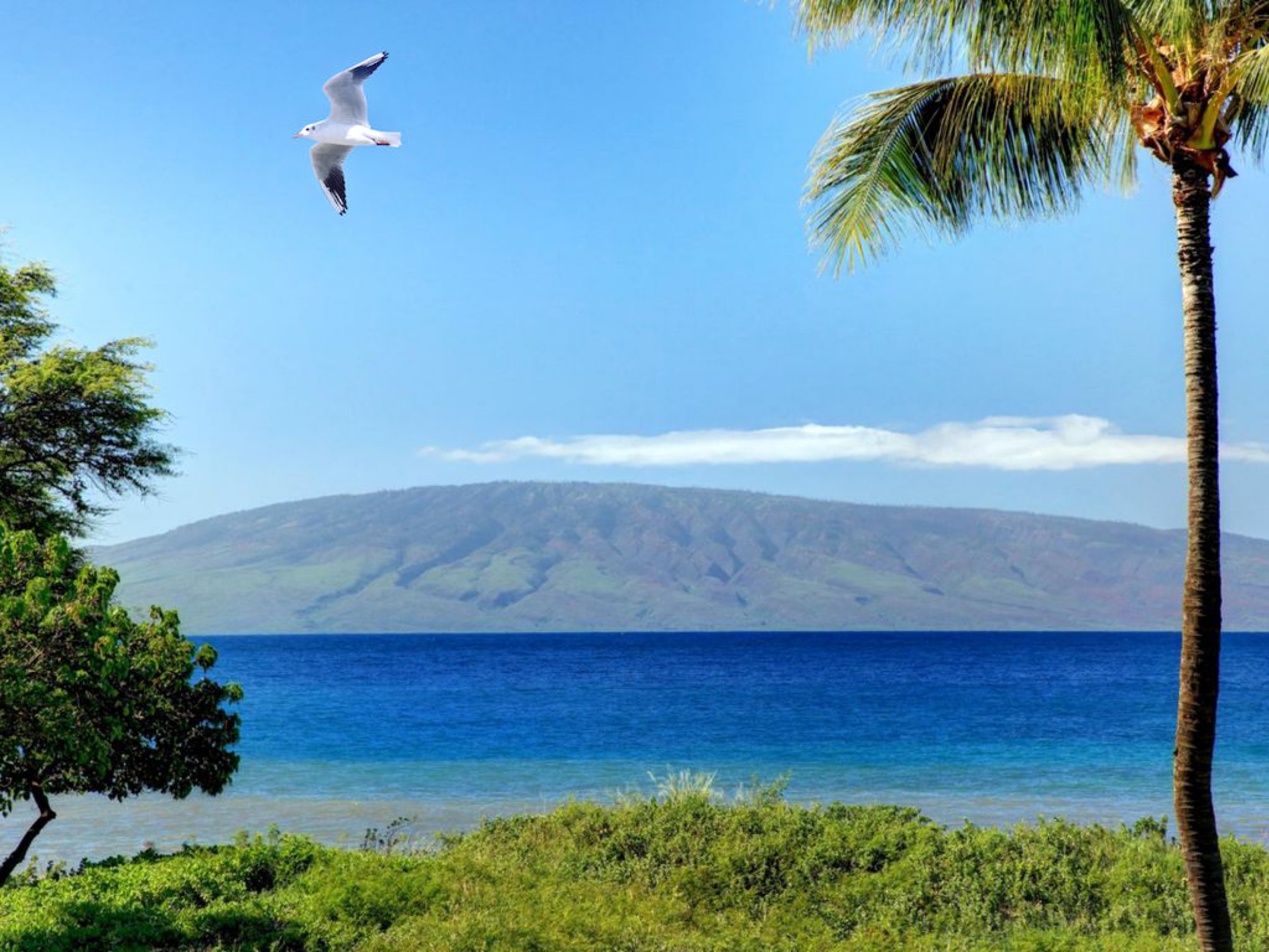
| Example Name | First Image | Second Image | Result |
|---|---|---|---|
| Seagull by the Bay | 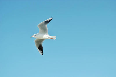 |
 |
 |
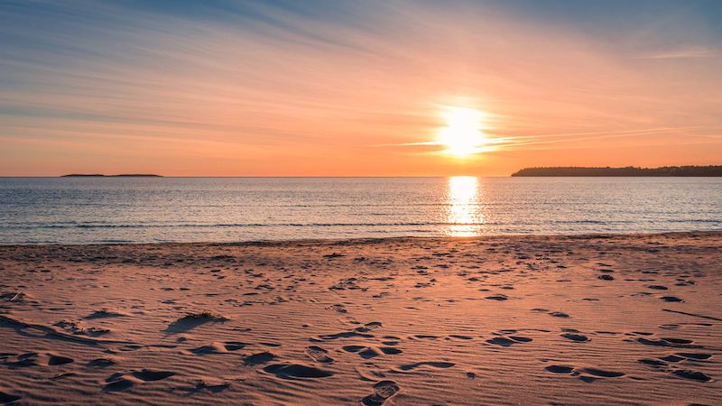
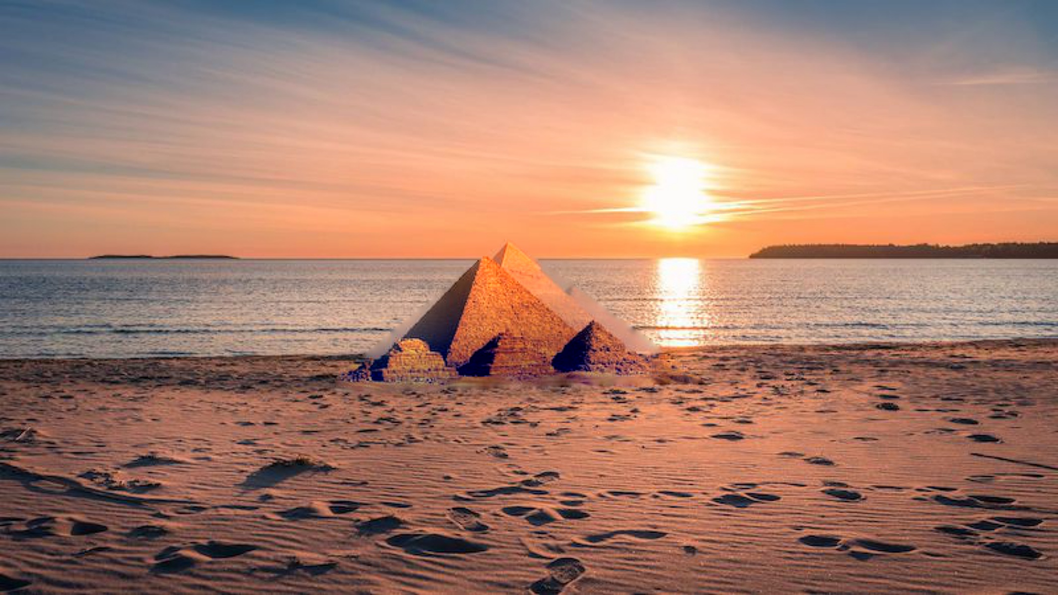
| Pyramid on a Beach | 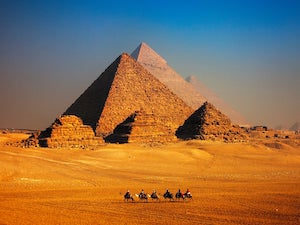 |
 |
 |
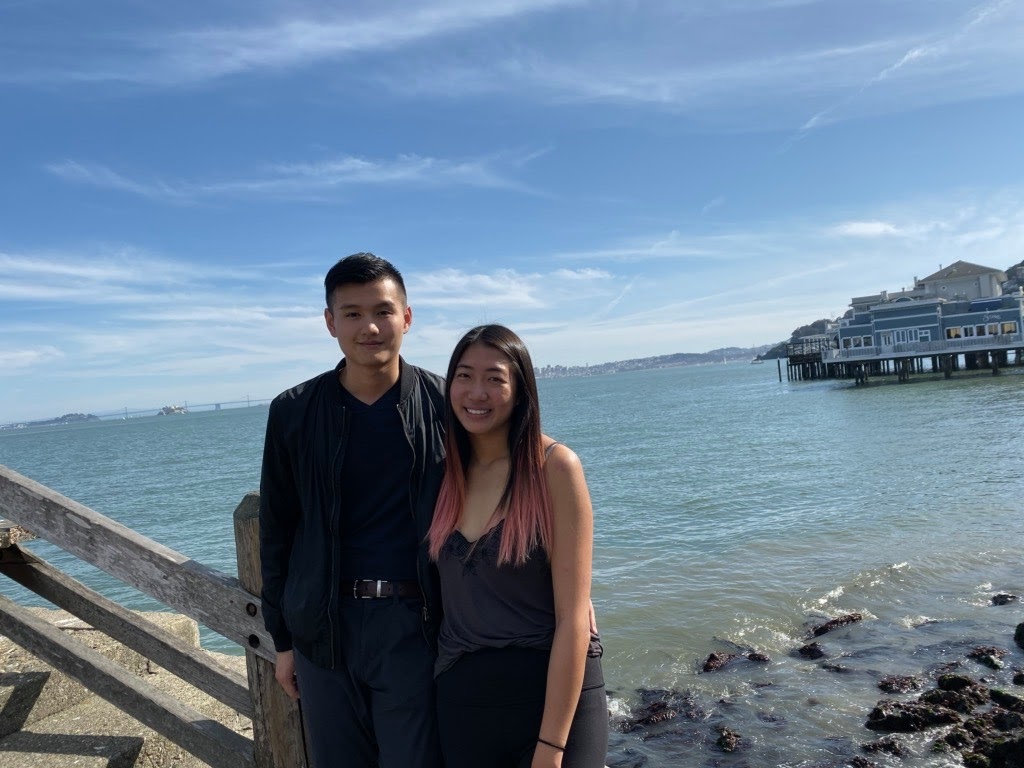
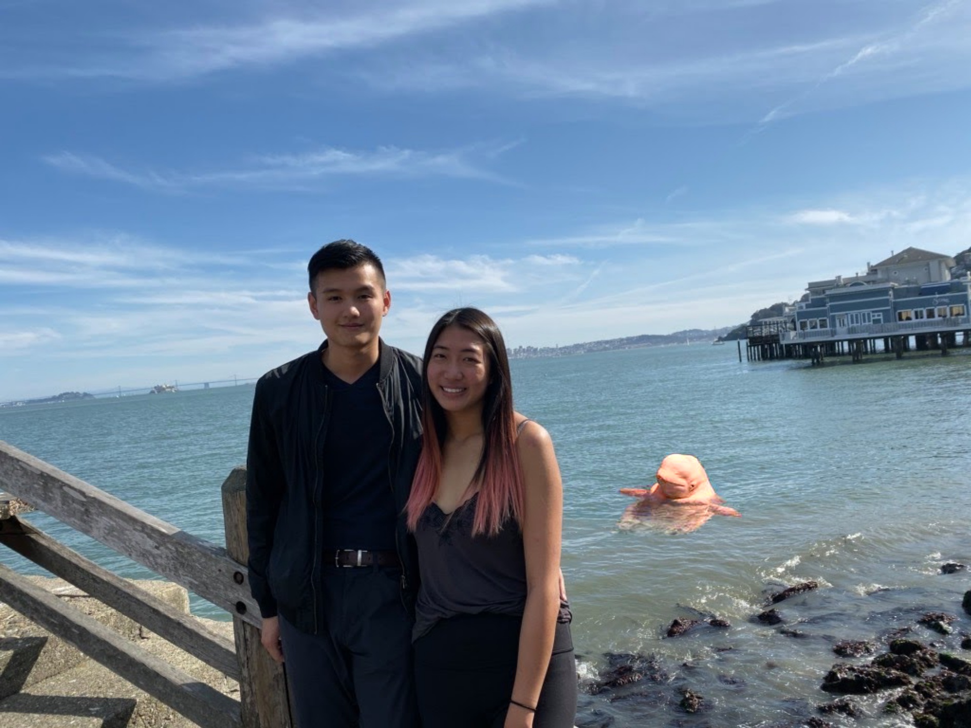
| Beluga in Marin | 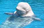 |
 |
 |
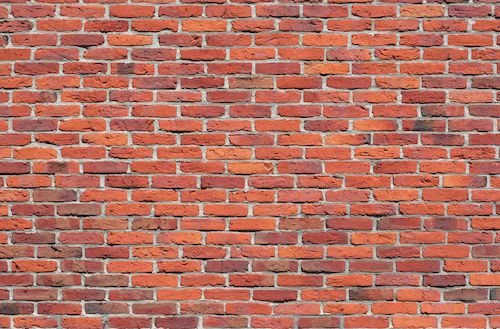
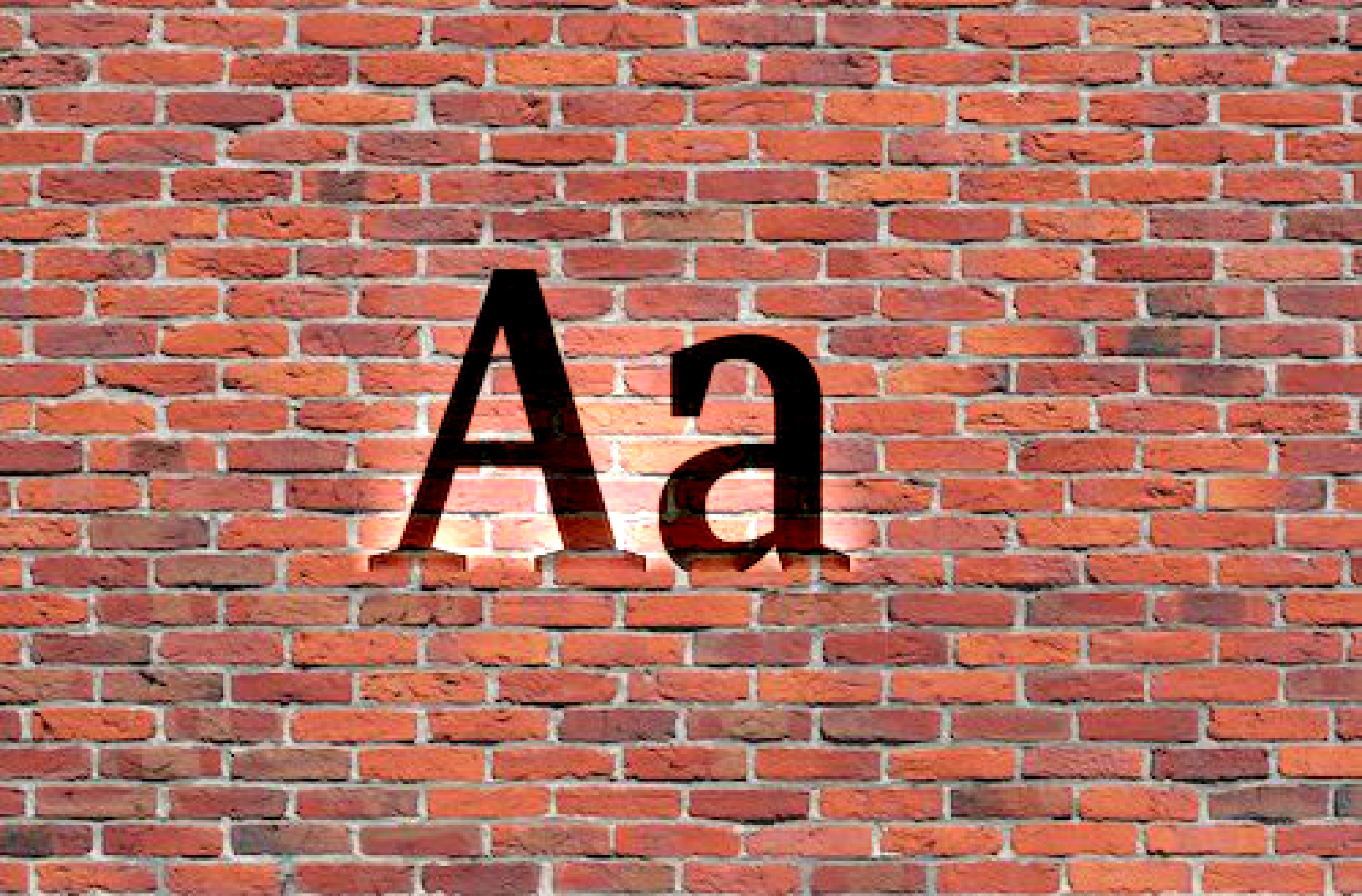
In the naive method of Poisson blending above, we could only honor the gradient for one image at a time. In other words, there is no way for us to include texture from both images in the same location. Using a mixed gradients method, however, we can emphasize the more extreme gradients from each image, which allows us to make things more interesting. In the below example, the image on the left is simple text on a white background. If we were to use the naive method, we would see a lot more of the text image's white background.
| Example Name | First Image | Second Image | Result |
|---|---|---|---|
| Writing on the Wall (Naive) |  |
 |
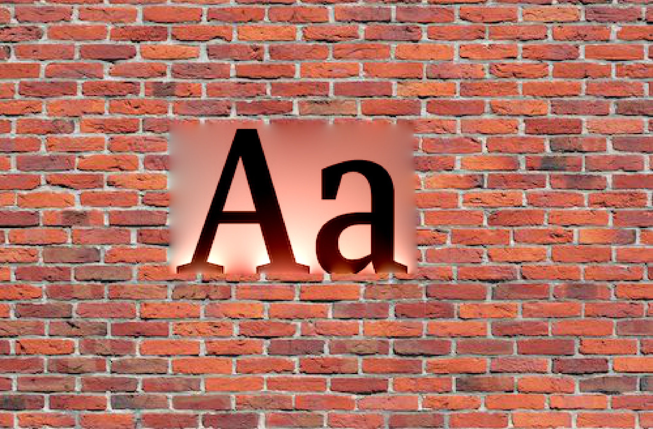 |
| Writing on the Wall (Mixed Gradients) | |
|
 |
I was pleased by most of the results. In particular, I found the mixed gradient strategy to be really interesting. Compared to Laplacian pyramids, Poisson blending seems to give much more flexibility by allowing us to define linear constraints in whatever way we want. The pyramid example is probably is worst result. I would attribute its relative failure to the fact that both the source and target images have a lot of messy gradients on the edges. The best result was unsurprisingly the seagull. In both the target and source images, the background was a clear blue sky.
We learned that using light-field cameras, which represent a scene from many slightly different angles, we can perform post-processing that would be unavailable in a standard camera. In particular, we can perform digital refocusing, allowing us to adjust focus to our liking. Using data from the Stanford Light Field Archive, we can translate the images relative to one another to focus on different depths of a scene. In the examples below, we repeatedly shift from focusing on the background to the foreground. In my code, I first find the center image, then shift all other images toward the center image by a variable amount. This variable amount is defined as the distance from each other image to the center image, multiplied by a parameter alpha.
| Example Name | Alpha range | Result |
|---|---|---|
| Chess | [-0.3, 1.0] |  |
| Bean | [-0.8, 0.3] |  |
| Amethyst | [-0.5, 0.5] |  |
In addition to shifting the focus between the background and the foreground, we can also adjust the effective aperture size by including more or fewer of the images captured. The intuition behind this is that with more images averaged, we see light rays captured from more angles, so the result is blurrier. In the other extreme, if we only take one image, then there is no blurring effect. In the examples below, we maintain focus on one area of the image, but we repeatedly adjust the aperture size to focus on more or less of the surrounding areas. In my code, I parameterized my function in terms of a radius in range 0 to 8: 0 means that I only care about the center image; 8 means that I include all the images.
| Example Name | Radius range | Result |
|---|---|---|
| Chess | [0, 8] |  |
| Bean | [0, 8] |  |
| Amethyst | [0, 8] |  |
I was surprised by how good the results were. Given that the images were taken from many different angles, I had intuitively expected there to be a lot of noise and perhaps mismeasured positions of the cameras. However, the camera positions are surprisingly reliable—I would not expect to be able to recreate this quality of data using just my own camera.