CS 194-26: Final Project
Akshit Annadi
Image Quilting
In this project, we explored how we could quilt portions of images together to accomplish texture synthesis and texture transfer
Texture Synthesis - 3 Methods
Texture synthesis is the creation of a larger texture image from a small sample. We explored three methods to do this.
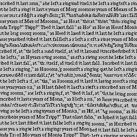
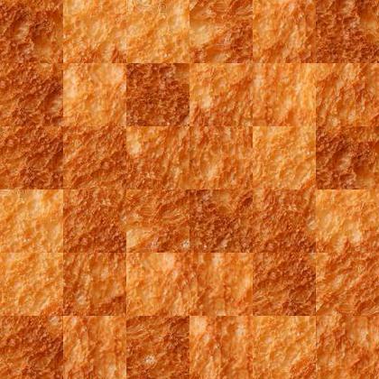
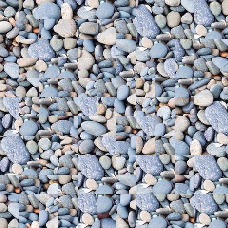
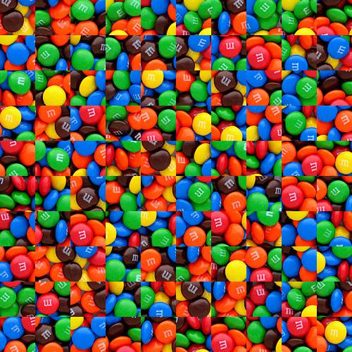
Randomly Sampled Texture
In the first method, we simply take the blank output image and randomly fill it in with patches from the source texture image until the entire output image is filled.
For most textures, this produces a broken texture with visible seams between patches.
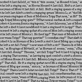
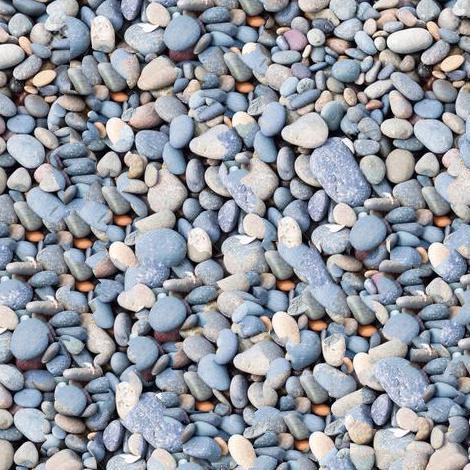
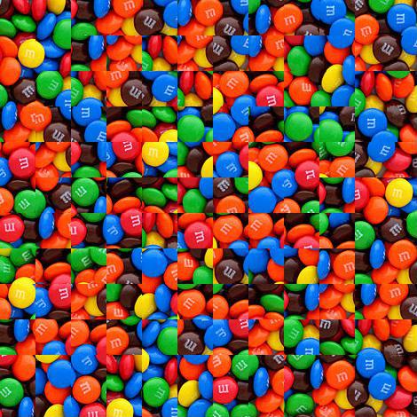
Overlapping Patches
In the second method, instead of randomly filling in patches, we find patches that overlap well with its neighbors that are already in the output image to avoid visible edges/seams. To do this,
we simply fill the output image patch by patch, but we add patches that overlap with the patches to its left and top in the output the best. We test out different patches and find the one that
has the lowest SSD distance in the overlap between its neighboring patches. Then we choose the lowest SSD patch or another patch that has a similarly low SSD and place it in the output image.
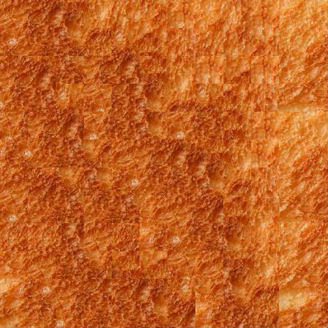
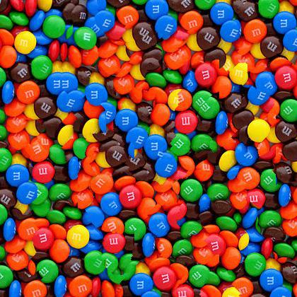
Seam Finding
In the third method, we largely build off the overlapping patches method. Once we find the best patch using the overlapping patches method, we don't simply replace the overlap with the new patch like in the method above. Instead, we
find the minimum cut path in the overlap and then stitch together the overlaps of the patches along the cut. An example of this can be shown with the following images:

Image 1

Image 1 Overlap

Image 2 Overlap

Image 2
The following shows the SSD distance between the two images in the overlap and the minimum cut along the path, both in the SSD image and the original image.

Overlap SSD Distance

Overlap SSD Seam

Original Image Seam

Stitched Overlap
Results
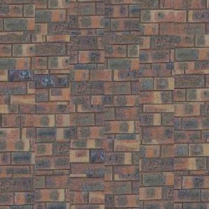
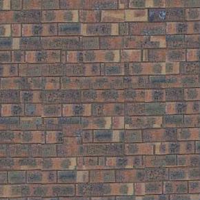
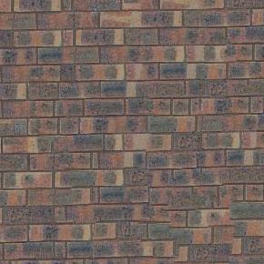
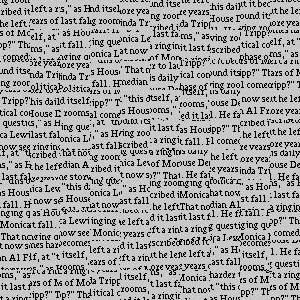
Here are the results of all 3 methods over 5 textures:

Bricks Texture
Words Texture
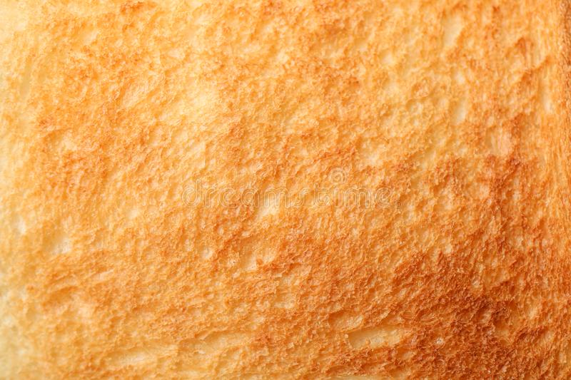
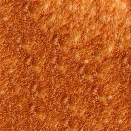
Toast Texture
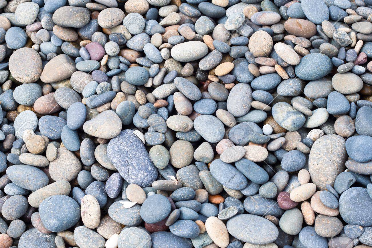
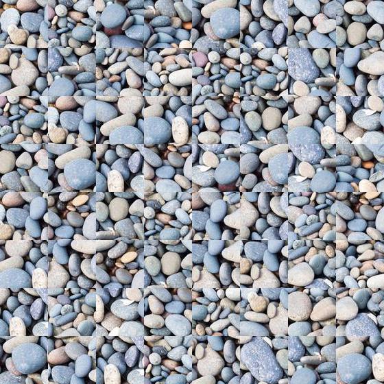
Stones Texture
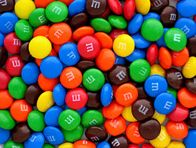
M&Ms Texture
Texture Transfer
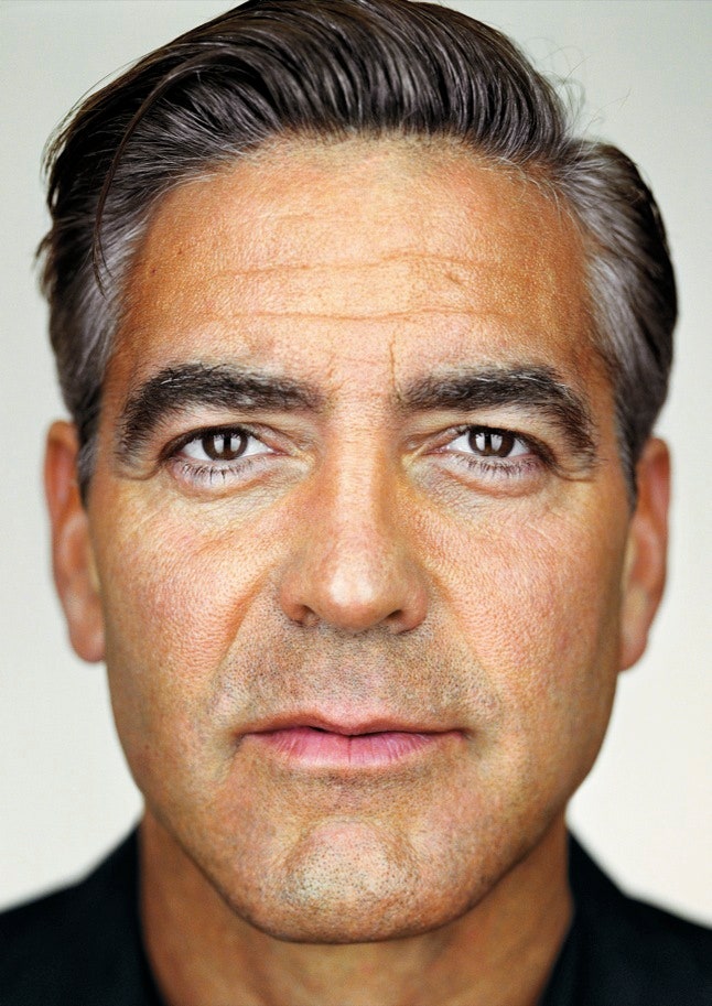
We can directly apply texture synthesis to a new application, texture transfer. Texture transfer is giving an object the appearance of having the same texture as a sample while preserving its basic shape. We do this by not only finding patches that blend
into surrounding patches like in synthesis, but ones that also match the corresponding patch in the desired output. To accomplish this, we only need to make one minor change to our existing synthesis algorithm. In addition to using the SSD
between the overlap in patches as a cost, we also add the SSD between the patch and the corresponding patch in the desired output. The results for three sets of images are shown below:
Texture
Target
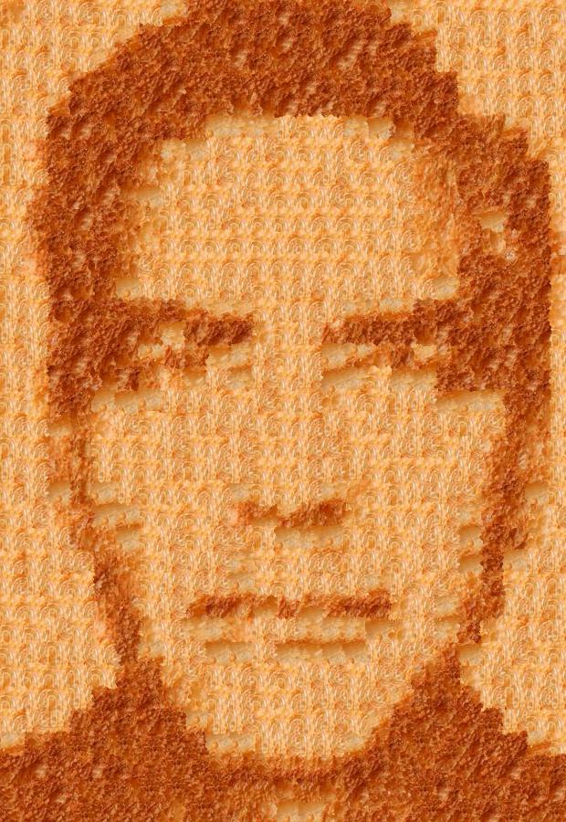
Clooney Toast
Texture
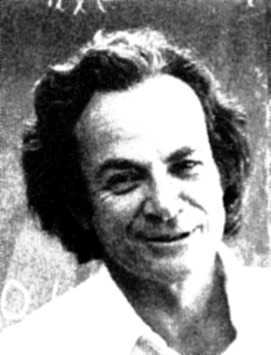
Target
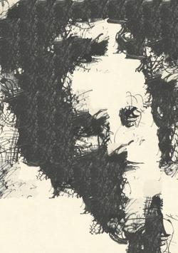
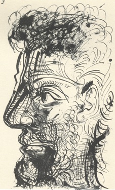
Portrait Sketch
Texture
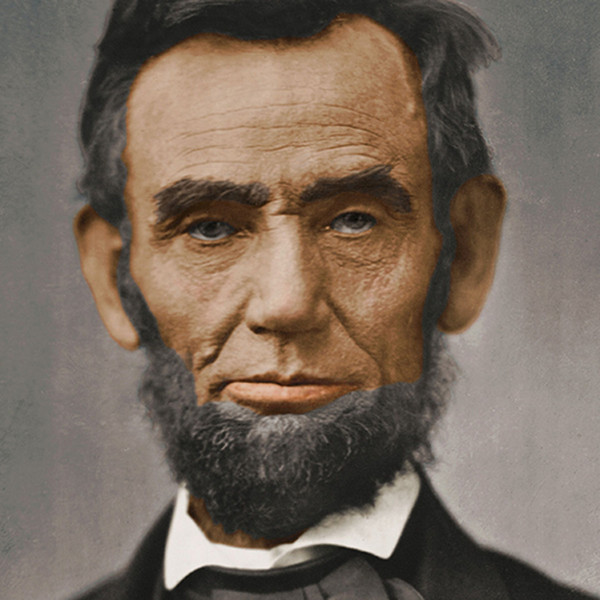
Target
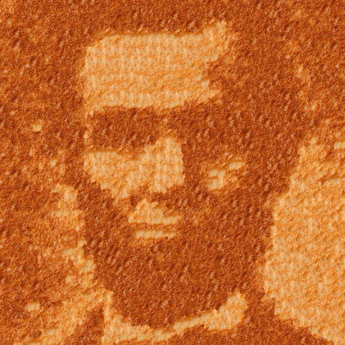
Lincoln Toast
Bells and Whistles
For the bells and whistles for this project, I made my own cut function. The given skeleton code was in matlab, which I had no background in, so I created my own in python(vertical_seam and horizontal_seam in common.py).
The functions worked by taking in the overlapped portions of two images, computing the SSD distance image, and then using a dynamic programming algorithm to go row by row in the distance image to find the minimum path
from top to bottom or left to right.
Light Field Camera
In this project, we used light field data to simulate depth refocusing and aperature adjustment on a scene. The light field data was in the form of a 17x17
grid of images. Averaging and shifting these images allowed us to simulate the photo effects.
Depth Refocusing
Averaging all the images in the grid without any shifting will produce an image which is sharp around the far-away objects but blurry around the nearby ones becasue the nearby objects change position
across the images. However, we can shift each image with respect to the center image(8,8) and compute a new average to simulate focus at different depths. The shift applied to the (i,j)th image is C *(i-8, j-8) where C is some constant.
Once we calculate the shift, we use np.roll to actually edit the images and then average them. The results for two datasets is shown below.
Average with no shift(C=0)
Average with C=3
Gif of shifts from C = -1 to C = 3
Gif of shifts from C = -5 to C = 1
Aperture Adjustment
Rather than changing the point of focus, we can simulate changing the aperture while keeping a constant point of focus. To do this, instead of shifting images, we take an average
of a varying radius(r) of images around the center. In my approach, for a radius r, we average the rxr grid of images around the center image. The following is the results for two datasets:
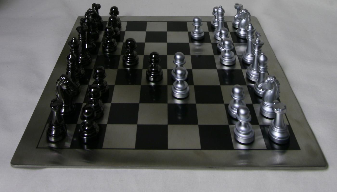
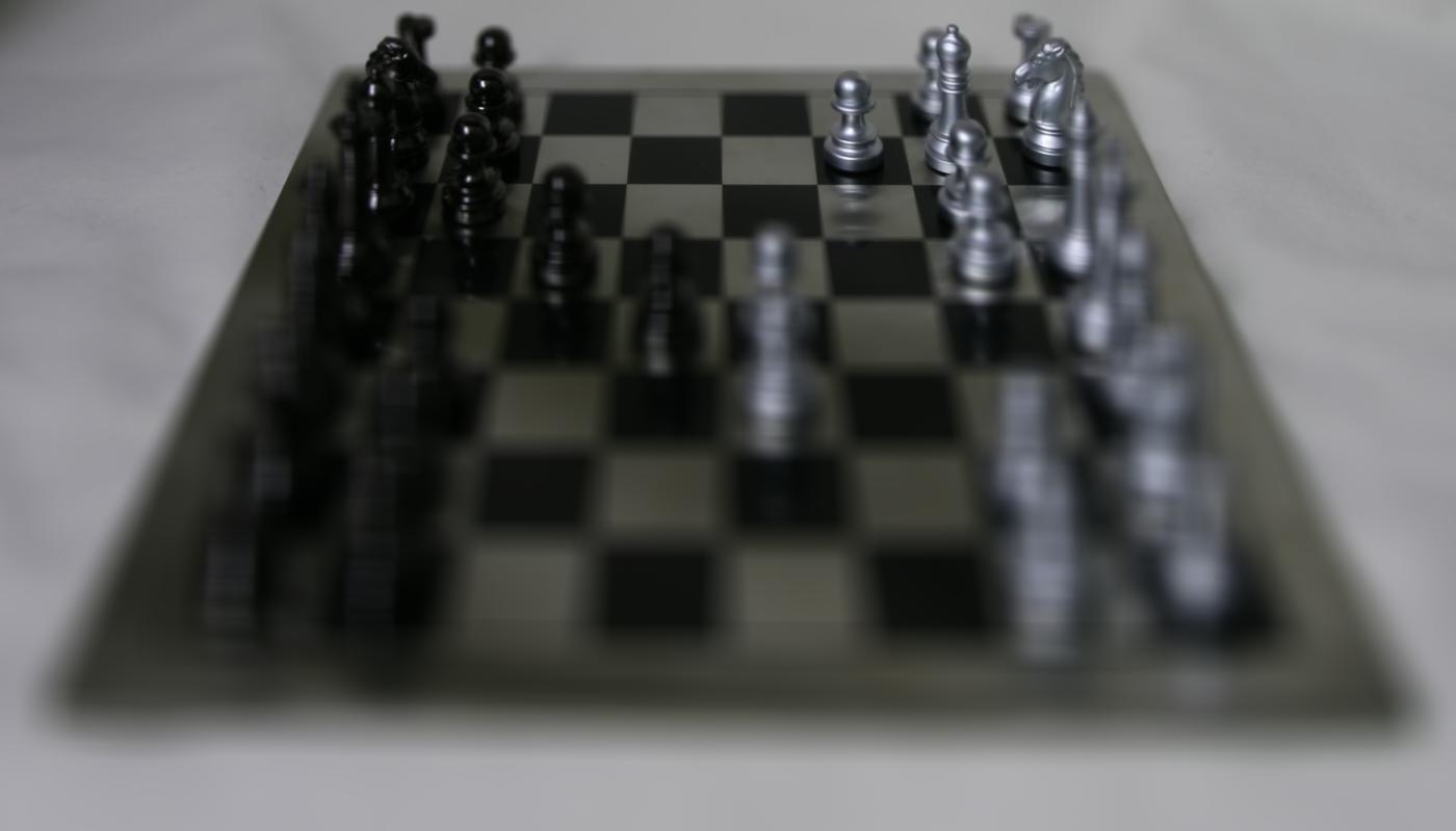
Chess data with r = 0
Focus point in the back
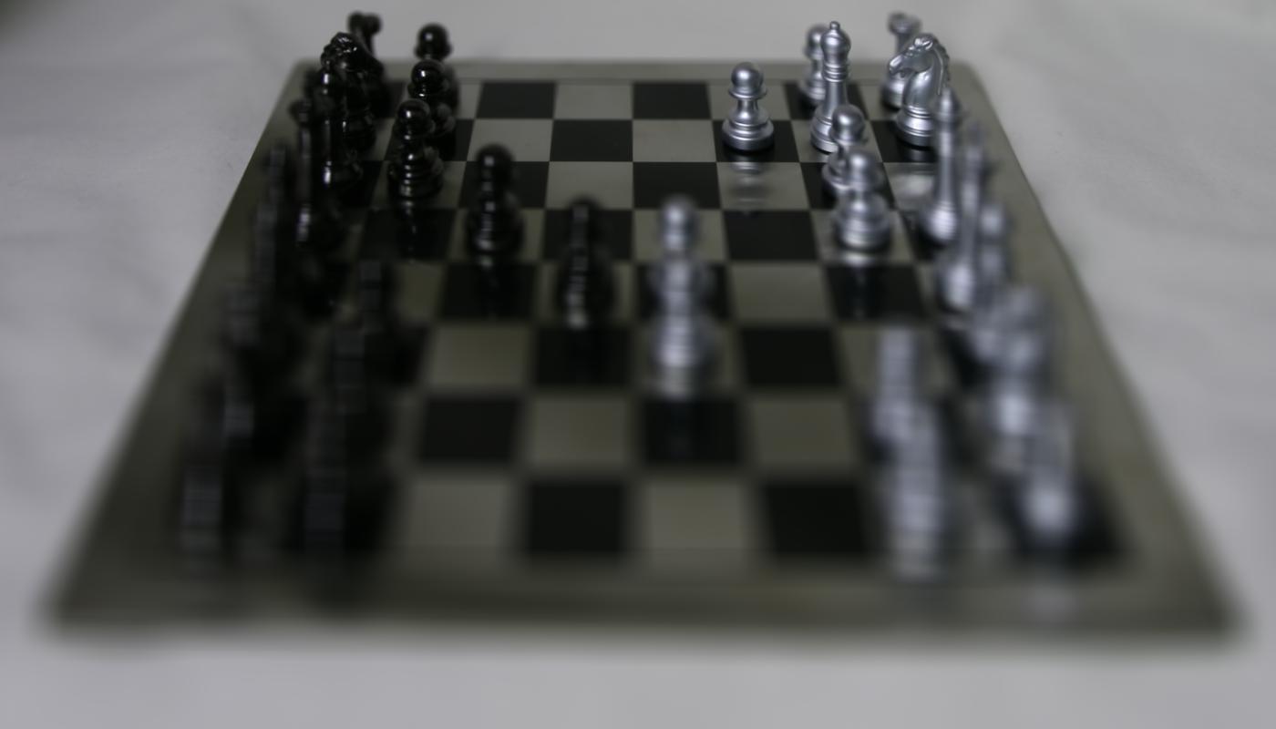
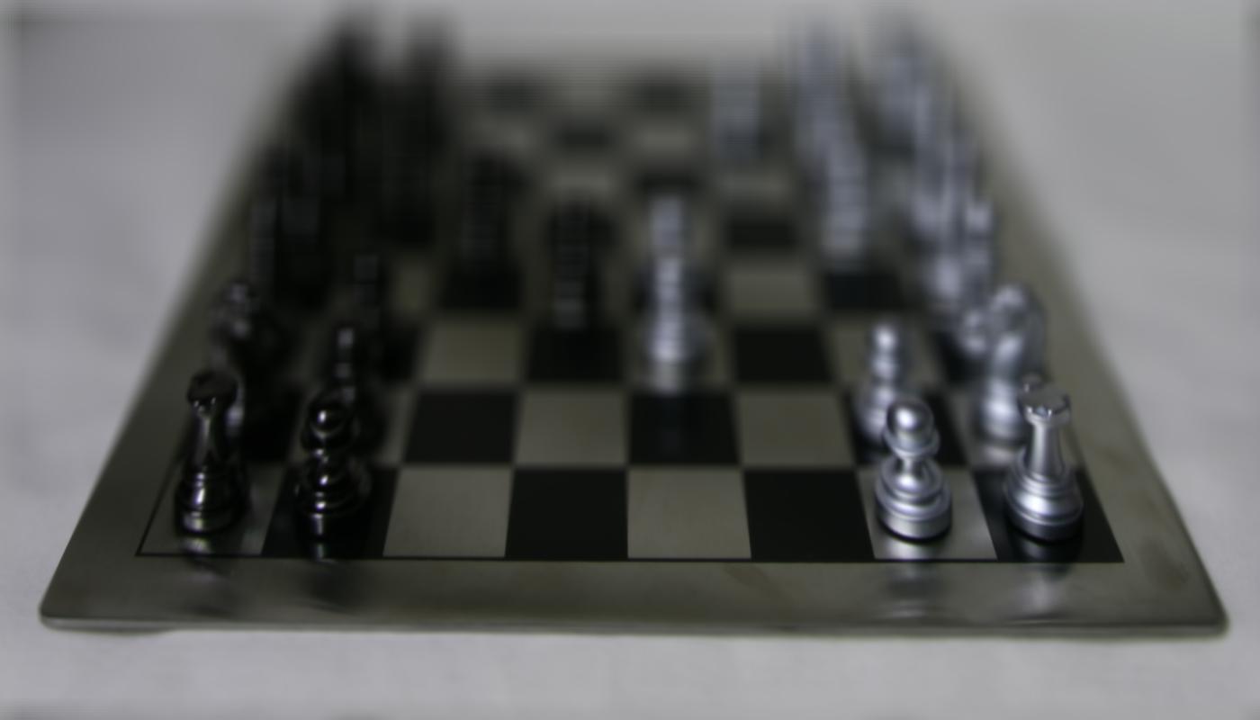
Chess data with r = 7
Focus point in the back
Gif of aperature simulation from r = 0 to r = 8
Focus point is in the back
Gif of aperature simulation from r = 0 to r = 8
Focus point is in the front
Learnings
It was fascinating to see that with a lightfield camera, you really do have enough data to simulate many different things in the processing of images that only seem to be variables of the position and setting of the camera.