CS194-26 Final Project - Eric Leong
Overview
For my final project, I worked on two pre-canned projects:
Image Quilting
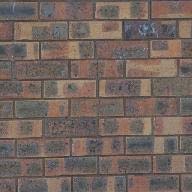
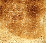
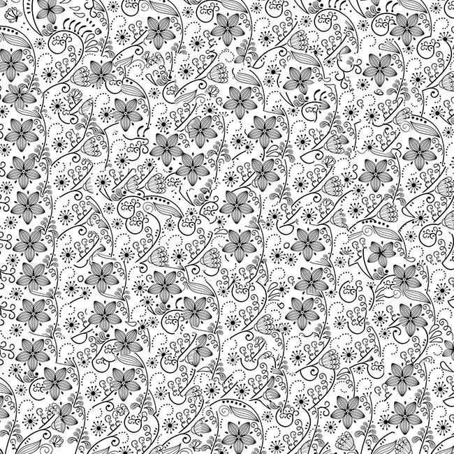
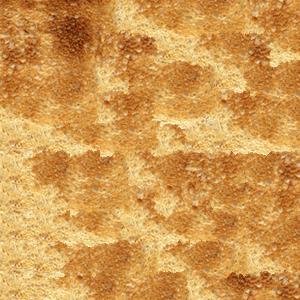
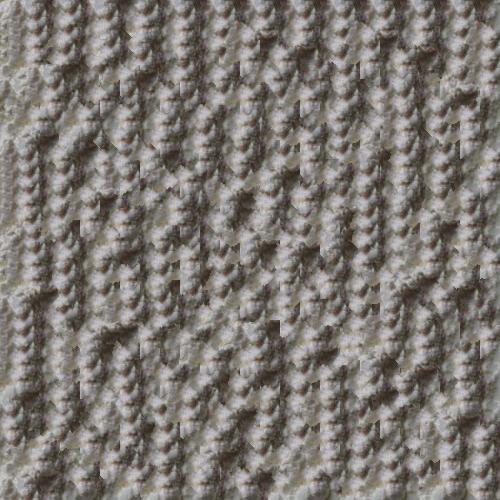
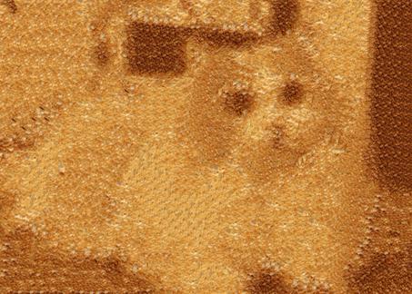
In this project, I worked on implementing the image quilting algorithm for texture synthesis and texture transfer. The algorithm is based on this paper. In texture synthesis, a larger texture image is created by combining many samples of a smaller texture image. We implement this with 3 different algorithms. In texture transfer, we use our methods for texture synthesis and add additional constraints to make the samples look similar to a target image.
Algorithms for Texture Synthesis
We perform texture synthesis using 3 different algorithms, starting off with simply combining randomly sampled patches without checking for compatability, adding overlap between patches to ensure that adjacent patches match decently, and using seam finding so to minimize the seams in the overlapping regions.
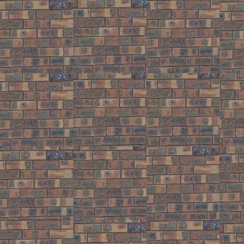
Random Patch Texture
Our first algorithm works by first creating an empty image of the desired size, then iteratively filling in the empty image with a randomly sampled patch (with size based on the user) from the source texture image until the image has been filled. In the regions of the image in which the entire sampled patch would not fit, i.e. the corners and edges, we simply truncate the patch so that it would fit.
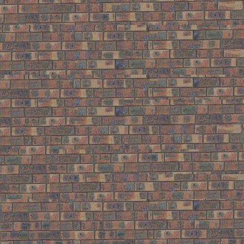
Overlapping Patches
From our first algorithm results, we noticed that there were very noticable "borders" or visual artifacts between adjacent patches. Instead of simply selecting any random patch from the set of possible patches from our source texture image, we first find a filtered set of patches based on how well the overlapping regions matches with the current image. Each of the patches will overlap by a predefined margin and we use the SSD cost function to measure how well the overlapping regions match. Our algorithm is now as follows:
- Compute a set of all possible candidate patches and their centers.
- Find the region of overlap of where the patch would be placed, and the one's that have already been placed.
- Compute the SSD of all candidate patches and the overlapping patches.
- Filter out any patches that have ssd that do not fall within our desired tolerance range: (ssd <= (1.0+tolerance)*minE)
- Select a random sample from the remaining patches.
- Paste the sample into the corresponding region in the texture result.
- Repeat steps 2-6 until image is filled to the desired output size.
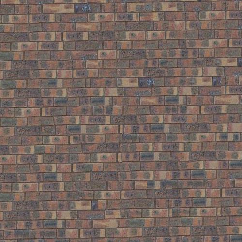
Seam Finding
The overlapping patches approach definitely improved our result, but there were still edge artifcats. We implement seam finding to find the min-cost cut in the overlapping region, and form a mask that determines which pixels we will use in the new patch that we found from step 5 of the previous algorithm. I created my own implementation of Seam Finding for Bell's and Whistles, which I describe in the Bell's and Whistles section.
Texture Transfer
Texture Transfer followed nearly the same approach as texture synthesis, with the exceptions that we now also take in as input a target image which we used to structure/model our output off of, and changed our cost function to account for similarity to the target image. Additionally, we create a new parameter alpha that determines the weight applied to the cost associated with the overlap region and the new cost for similarity to the target region. Our algorithm is now as follows:
- Compute a set of all possible candidate patches and their centers.
- Find the region of overlap of where the patch would be placed, and the one's that have already been placed.
- Compute the SSD of all candidate patches and the overlapping patches.
- Blur the target image (intensity image) and the candidate patches.
- Compute the SSD between the candidate patches and the corresponding region in the intesity imagae.
- Compute the resulting cost value: alpha*SSD_overlap + (1-alpha)*SSD_intensity
- Filter out any patches that have ssd that do not fall within our desired tolerance range: (ssd <= (1.0+tolerance)*minE)
- Select a random sample from the remaining patches.
- Paste the sample into the corresponding region in the texture result.
- Repeat steps 2-9 until image is filled to the desired output size, which is now the size of the target image.
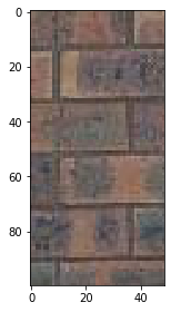
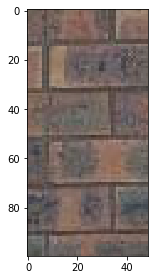
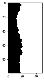
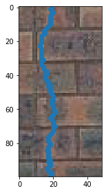
Bell's and Whistles: Seam Finding Implementation
Given a randomly sampled patch, we compute an error surface which is the ssd over channels of the sampled patch and the region for placement. There were 3 scenarios which we had to account for: vertical overlaps, horizontal overlaps, vertical and horizontal overlaps. We implemented a dynammic programming algorithm which takes in the error surface and finds the minimum cost path along the surface. We then used the minimum cost path to generate a mask containing the boundary in which we would use the pixels of the newly sampled patch. Thankfully, the process of seam finding was symmetric for vertical and horizontal overlaps, so we simply just implemented for the vertical direction and for the horizontal path, just used the vertical path method but transposed the input and the output. For the patches that overlapped in both, we individually computed the mask for the vertical and horizontal path, then combined them simply as follows: mask_h @ mask_v. Once we've found the masks, we can easily apply them to our sampled patch and paste it onto our texture result. The following images show the seam finding process for a pair of patches. In the mask, the white pixels denote pixels of value 1, meaning that we will use the corresponding pixel on the right patch in the overlapping region. As one can see, the algorithm works like a cookie cutter through the overlapping region to make the split.
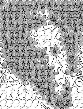
Texture Synthesis Results
Comparison between methods
Other Results


Texture Transfer Results
Varying Patch Size and Tolerance
Varying Texture
Other Results
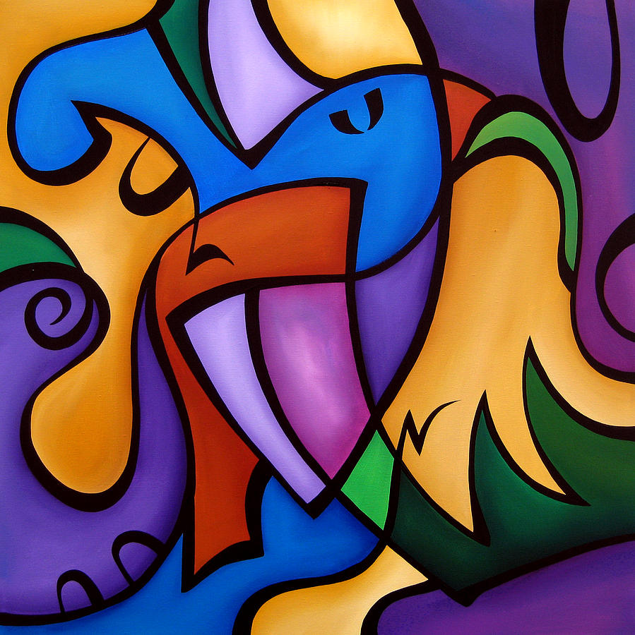
Neural Algorithm of Artistic Style
For this project, I worked on implementing the algorithm described in A Neural Algorithm of Artistic Style. The main idea that the paper elaborates on is that deep neural networks can be used as powerful tools for their perceptual abilities within the convolutional layers, powerful enough to separate content and style in images. The author then describes an artificial system that utilizes neural representations to separate and recombine content and style of arbitrary images, providing a neural algorithm for transferring artistic style.
Algorithm
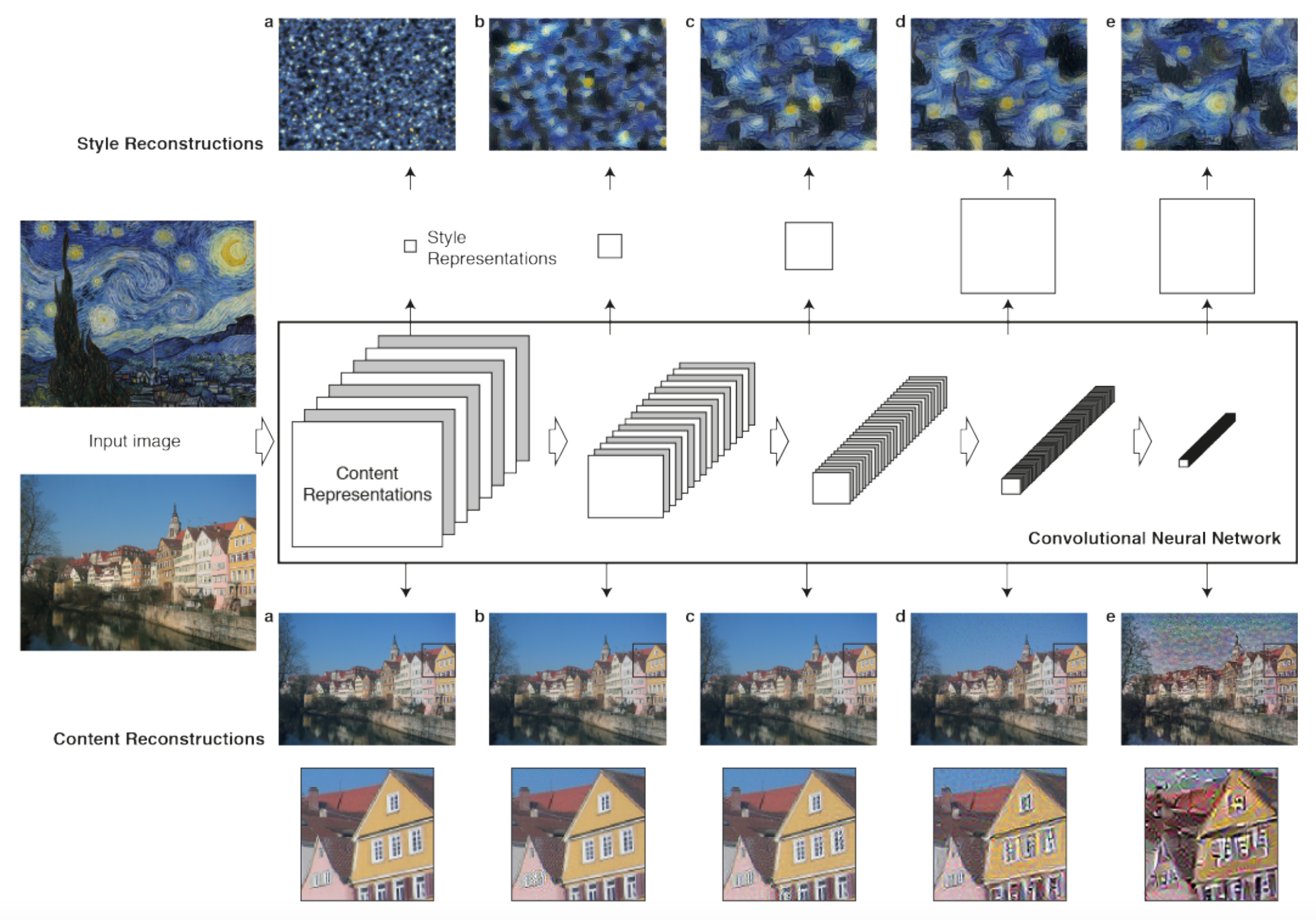
As an overview, the algorithm works by separating content and style representation in an image independently, using a deep neural network. As we move onto deeper convolutional layers in the network, we would notice that reconstructions of the original image would become less detailed as only the higher leveled features would be retained. As stated in the paper, "The style representation computes correlations between the different features in different layers of the CNN." The figure from the paper provides a great summary.
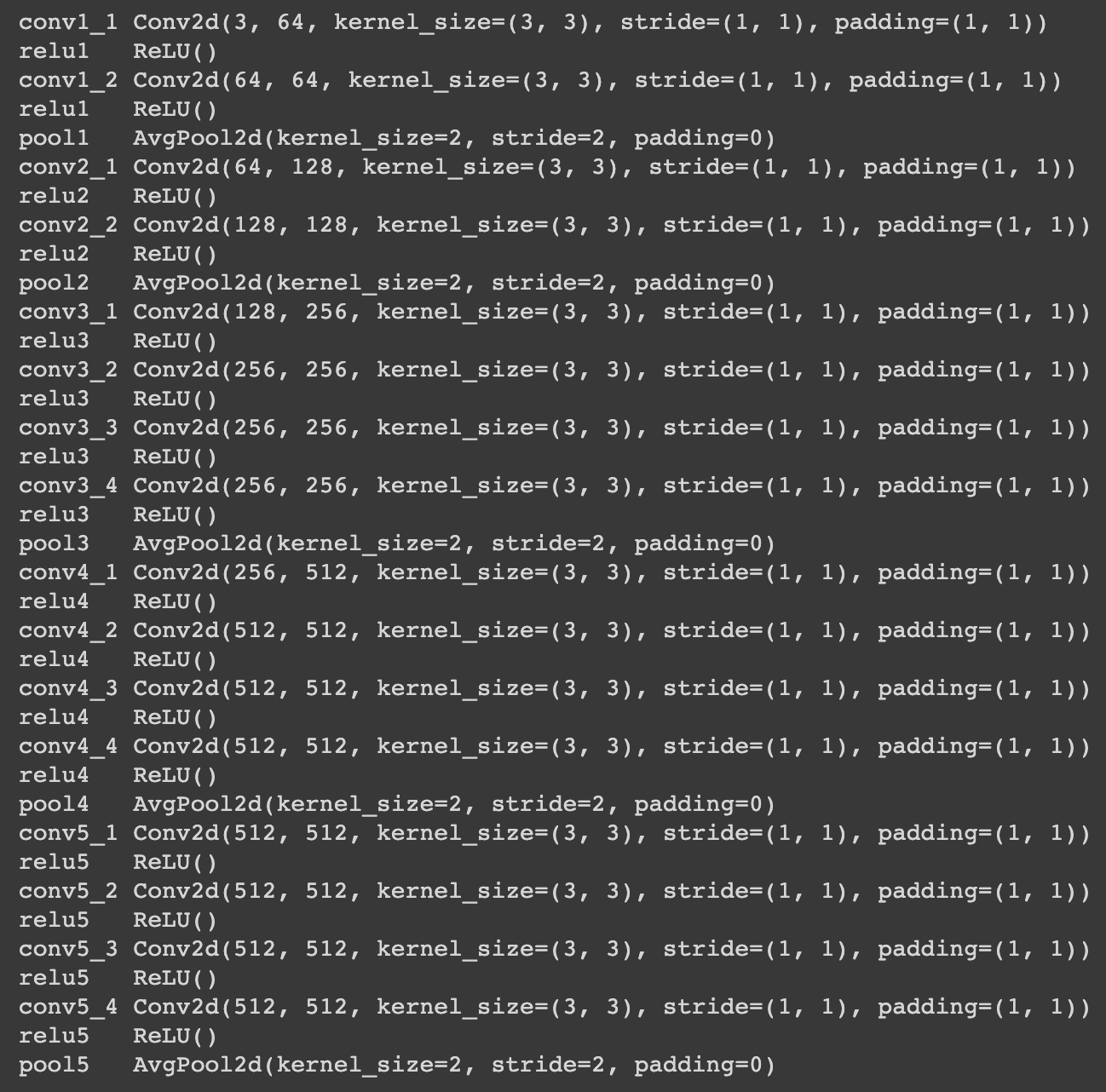
For the neural network, we followed the paper exactly and usesd a pretrained VGG-19 model with average pooling instead of max pooling and without any of the fully connected layers for the CNN.
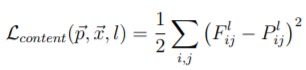
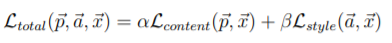
Once we have our neural network setup, we can work on the essence of the algorithm described in the paper, which uses gradient descent to reproduce an image by minimizing a certain loss function. We introduce 2 types of loss: content loss and style loss. p and x represent the original image and the image that is generated, P^l and F^l their feature representation at a layer l, A^l and G^l their style representation.
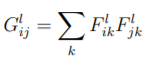
The correlation between feature responses between different layers, used for style representation, is computed using the Gram matrix.
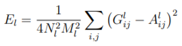
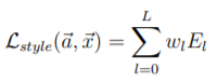
Finally, we define a total loss function, weighted by hyperparameters α and β, which we set depending on our images as a lower ratio of α / β would emphasize style representation significantly more.
Gradient descent will aim to minimize the total loss function to find the optimal pixel values for our image, and we utilized the L-BFGS algorithm as our optimizer. Similar to the paper, we matched the content representation on layer conv4_2, and the style representations on layers conv1_1, conv2_1, conv3_1, conv4_1, and conv5_1. I fixed my α value (content loss weight) to 1, and adjusted β value (style loss weight) accordingly. Number of epoch/iterations of gradient descent also varied by image.
Results
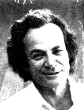
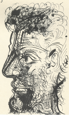
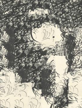
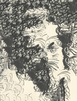
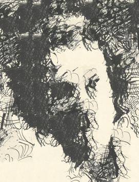
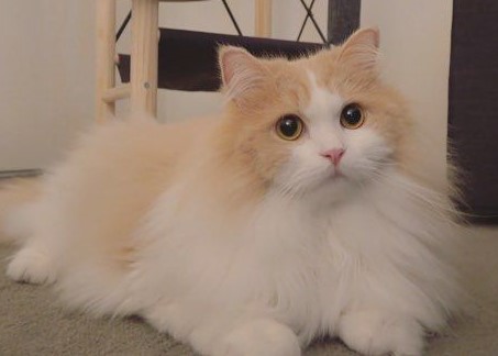
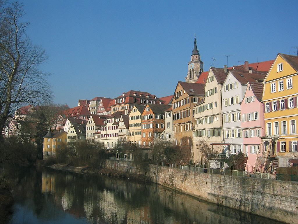
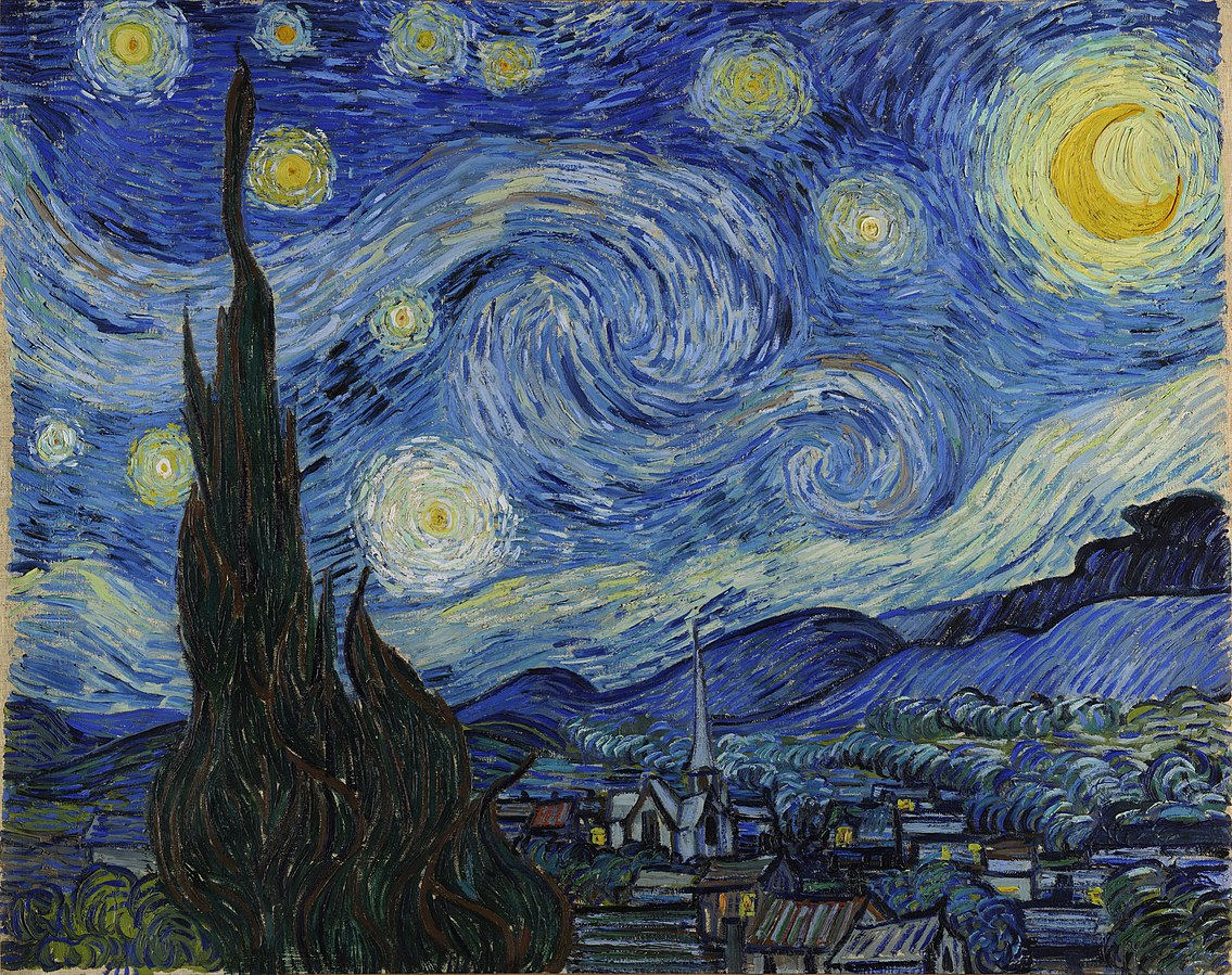
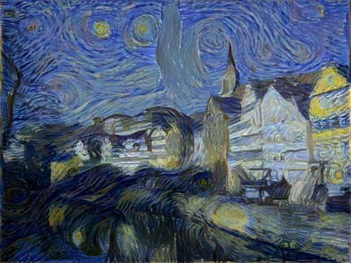
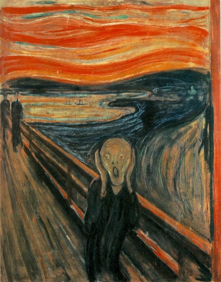
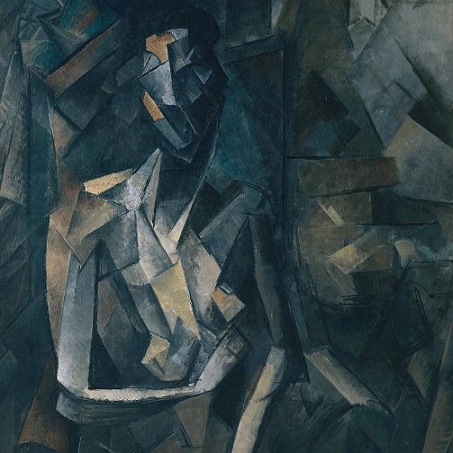
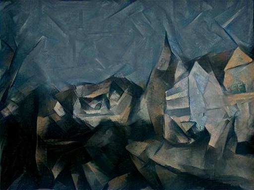
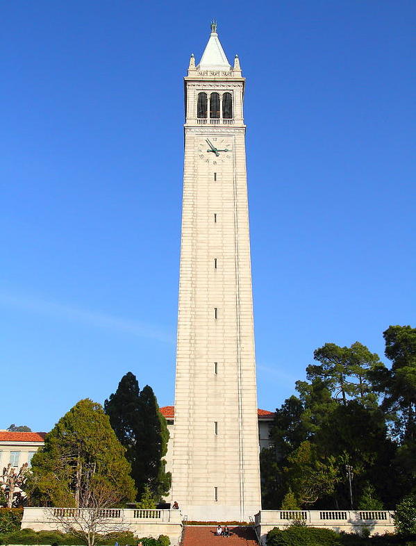
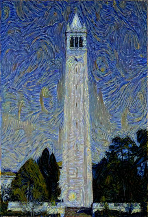
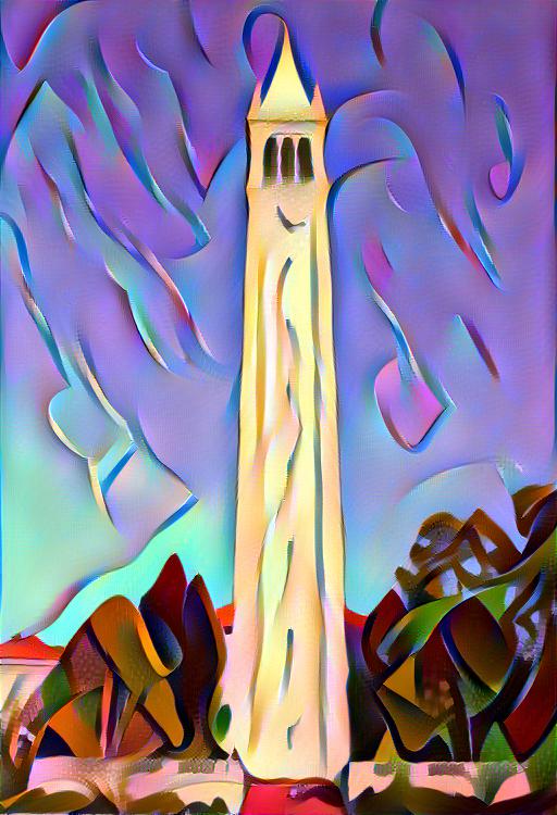
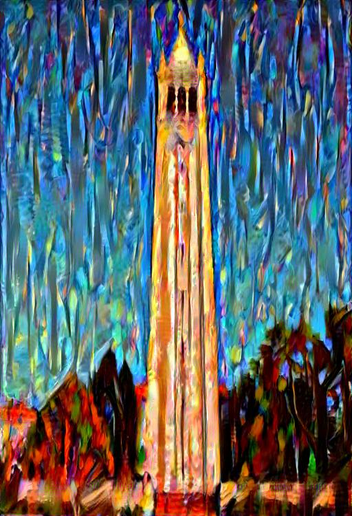
I first attempted to reproduce the results from the paper, using the "Tuebingen Neckarfront" image as the content image and using various style images. The results turned out quite nice! Each of them, when running for enough epochs and using the β used by the authors, matched the results from the paper quite well.
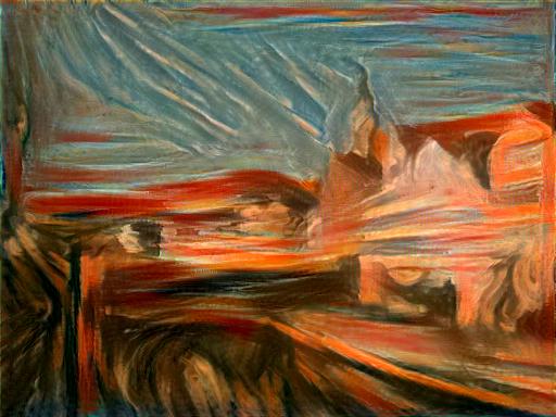
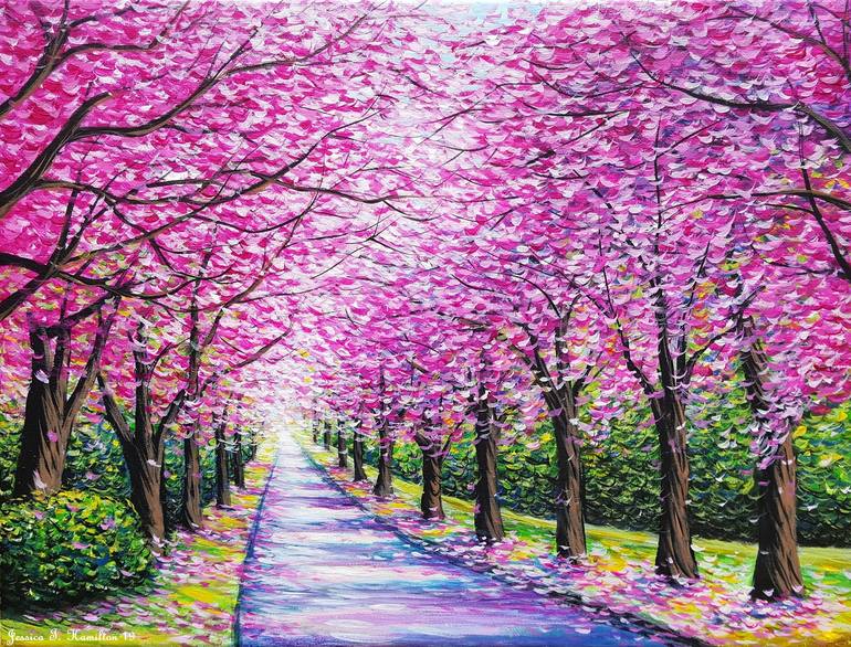
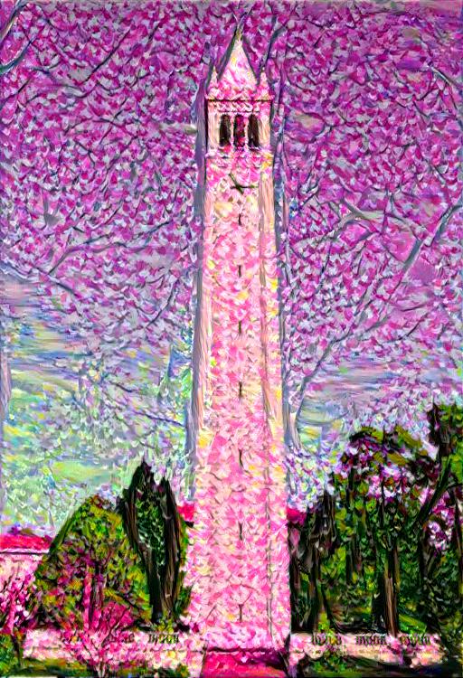
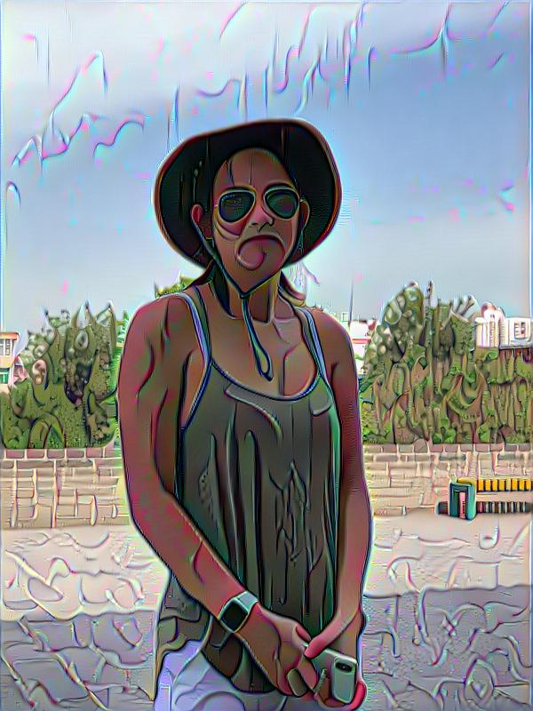
I then used the algorithm on a bunch of other images for fun, and most of them turned out really nice!

Failure Case
I was very curious as to whether it'd be possible to capture the style of cartoons, such as Family Guy, into an image. Unfortunately, my experiment didn't go too well and you can see that the result doesnt not have almost any of the artistic style in the style image. I suspect this has to do with the lack of core stylistic elements in the style image that is found in art pieces I've tried. As a result, the neural network does not develop a strong style representation of the image.

Final Thoughts
I enjoyed both of these projects a lot; these were probably my 2 favorite projects of this class. They were both very interesting and fun to work on. This class overall was an amazing class, and probably one of my favorite classes I've taken at Cal. It was a fascinating journey andn I appreciate the work Professor Efros and staff has put into the course.