CS194-26 Intro to Computer Vision and Computational Photography Final Project

For one of my final projects I have decided to re-implement the neural style transfer paper by Gatys et. al. This was a really fun project however I had some trouble getting the same results as the authors of the paper. This is probbaly because they don't specify every detail along the way so perhaps our algorithm to perform gradient descent is different. Additionally, I perform some data augmementation by performing random crops to get square content and style images.

Neural Network Implementation

First of all, I defined two "dummy" layers that I call Loss_c (content loss) and Loss_s (style loss). To implement the nerual stye transfer we need to compute the feature maps of the input image after specific convolutional layers and then based on whether we decided that layer to be a content identifying layer or style identifiying layer we want to pass this feauture map to an appropiate loss function. The network in quetsion is VGG19, which I downloaded (pretrained) from pytorch. The paper refers to layers such as conv4_2 -> this is the 2nd convolutional layer after the 3rd max pool operation. Additionally, the paper mentions that we should have a content loss function after the conv4_2 and style losses after conv1_1, conv2_1, conv3_1, conv4_1 and conv5_1.

My strategy was to then create modules called loss_s and loss_c that I could slip into the network into desired places and have their forward method simply be return input. This way they don't change the network but we can compute losses for every input that is passed to them. For example, as I'm iterating through the network layers I can keep track of what the name of each conv layer is so when I see conv4_2 I know I need to place after it a content loss module.

For the content loss module is pretty straightforward to compute the loss. We take in an input from the previous layer and compute it's feature representation (i.e. compute the filter response of the image at this layer's learned filters) then we perform a standard mse loss between this filter response and the filter response of the target image (the target image is simply the output of the model up to this specific layer when we pass in the content image). I actually tried experimenting a bit here and changed the sum of squared errors loss to l1 loss and got slightly smoother results.

The style loss is a bit more convoluted (no pun intended). The idea is the same as for the previous loss in the sense that we insert this loss module in between layers, in particular as the authors of the paper described we insert the style loss module in between the first convolutional layer after every max pool layer. At a high level the loss is essentially the same, we want to have a mse loss that will tell us how "close" the output of the networ up to this layer (aka the input to the loss layer) is to the output of the model up to the current layer when we pass in the style image. Basically, take the output of the model when you pass in the style image, and take the output of the model when you pass in the input image, we want these two outputs to be as close as possible in terms of style/texture. The problem however is we need to find a way to quantify the texture/style of an image. This is where the gram matrix comes into play. To my understanding the gram matrix basically computes a matrix of corrrelations between the filter responses of a specific layer. It can be easily computed by taking inner products of the rows of the feature map. This can easily be parallelized by returning FF^T, where F is the feature map. The paper then normalizes the entries of this gram matrix by dividing by the total number of feature entries (num_features * cols * rows). Now that we have the gram matrix setup we can use this as our input to the loss function.

Please note, in both loss layers I ended up switching from mse loss to l1 loss, I noticed the output was a bit better with this loss function.

Architecture

As the paper suggested I removed the final fully connected layers, here is my architecture. Please note the very first layer named normalization is simply to perform the aforementioned normalization that was used to train the netrowk by pytorch.

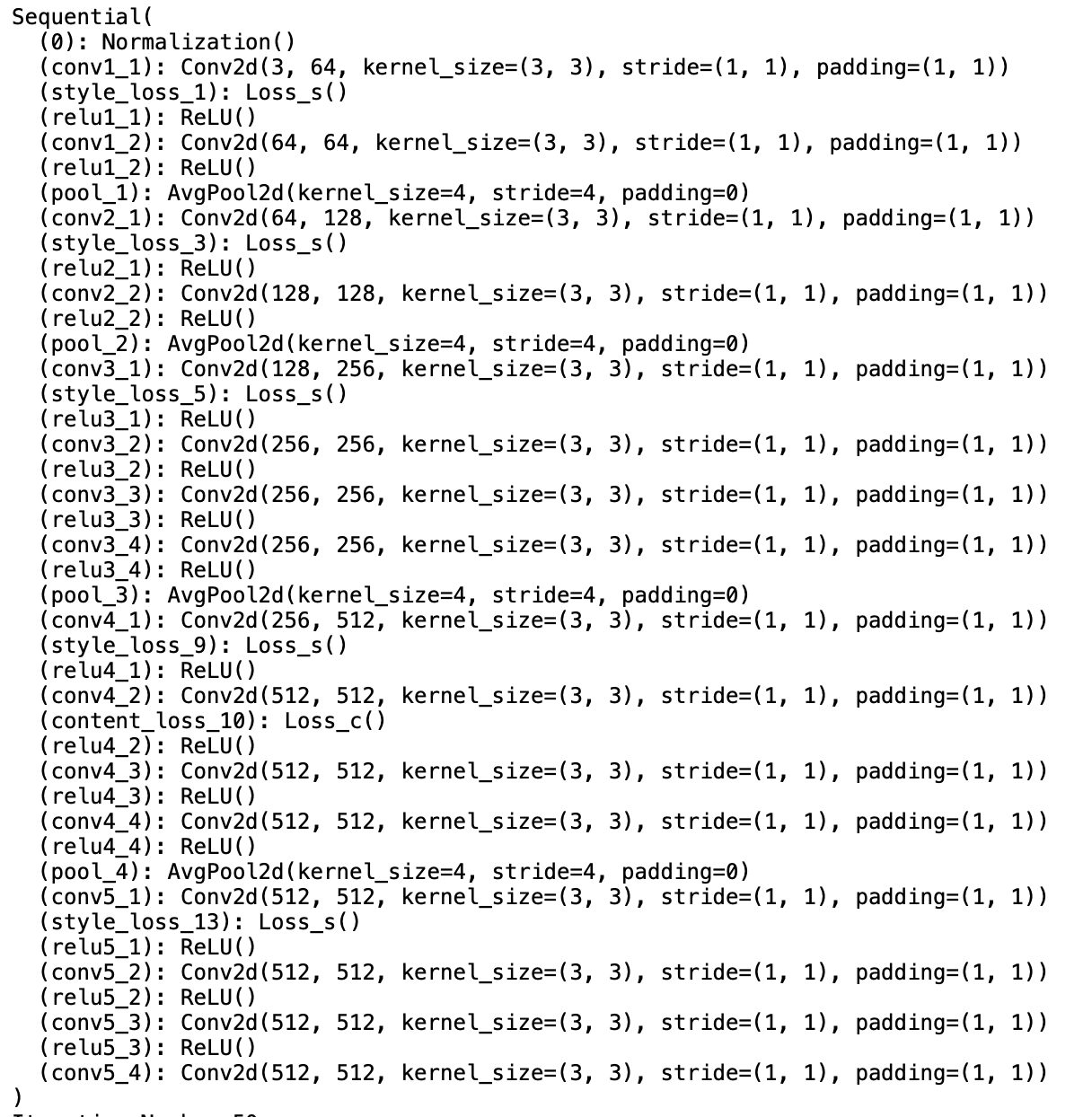
Performing the Style Transfer

Using the above network I create a "master loss function" which is simply the weighted sum of the two loss functions. The style loss is the average of the various loss functions at different stages of the network. I then run the adam descent algorithm for 800 steps to optimize this master loss function and the final step returns the desired image. I varied the learning rate and weights for each picture since they changed results (sometimes drastically). Most of the learning rated were in the 1e-2 to 1e-3 range. The style and content weights changed a lot also. Sometimes, I had to make the ratio of style weight : content weight > 1e4 (that was the value the paper used).

Neckarfront Results

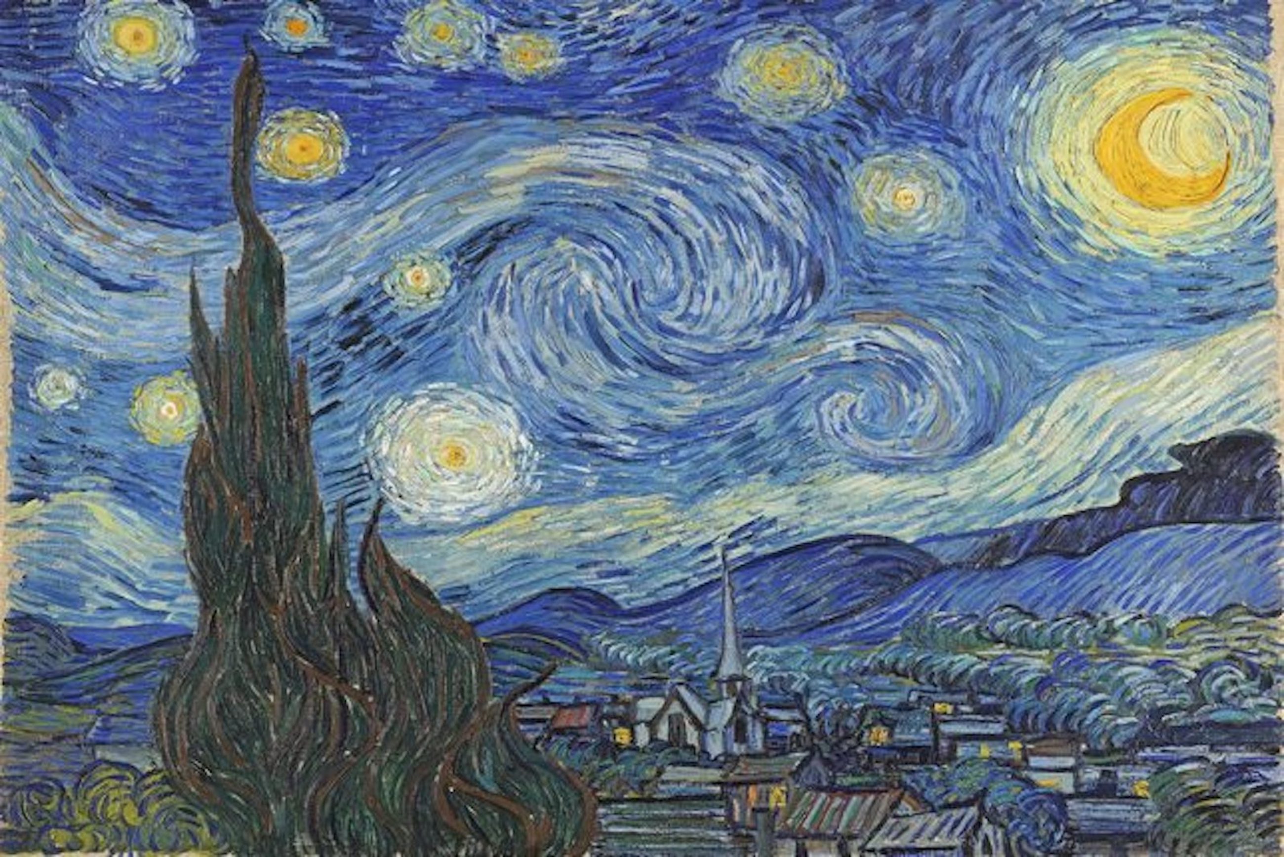
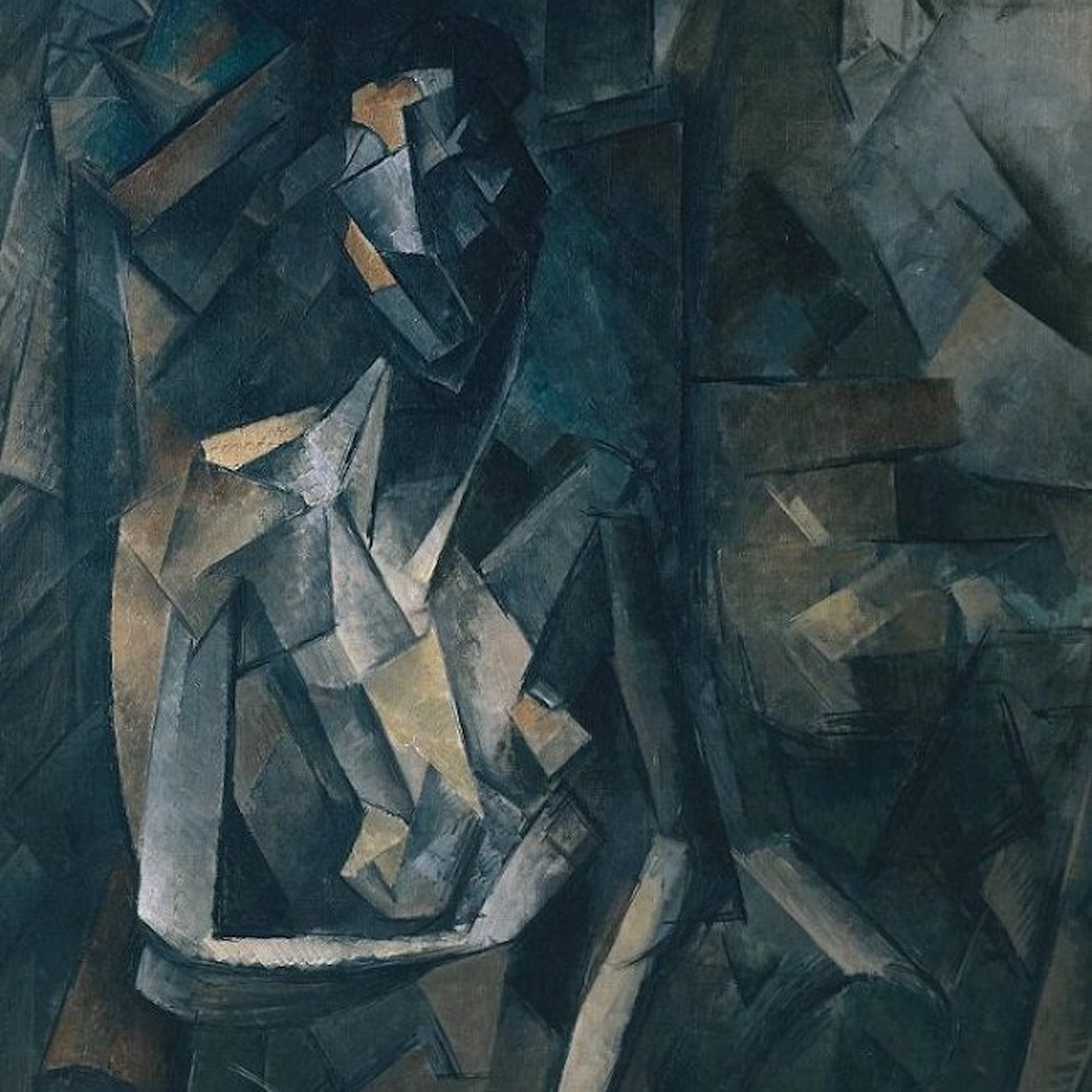
Here is the original Neckarfront image as well as the three styles I picked from the paper.

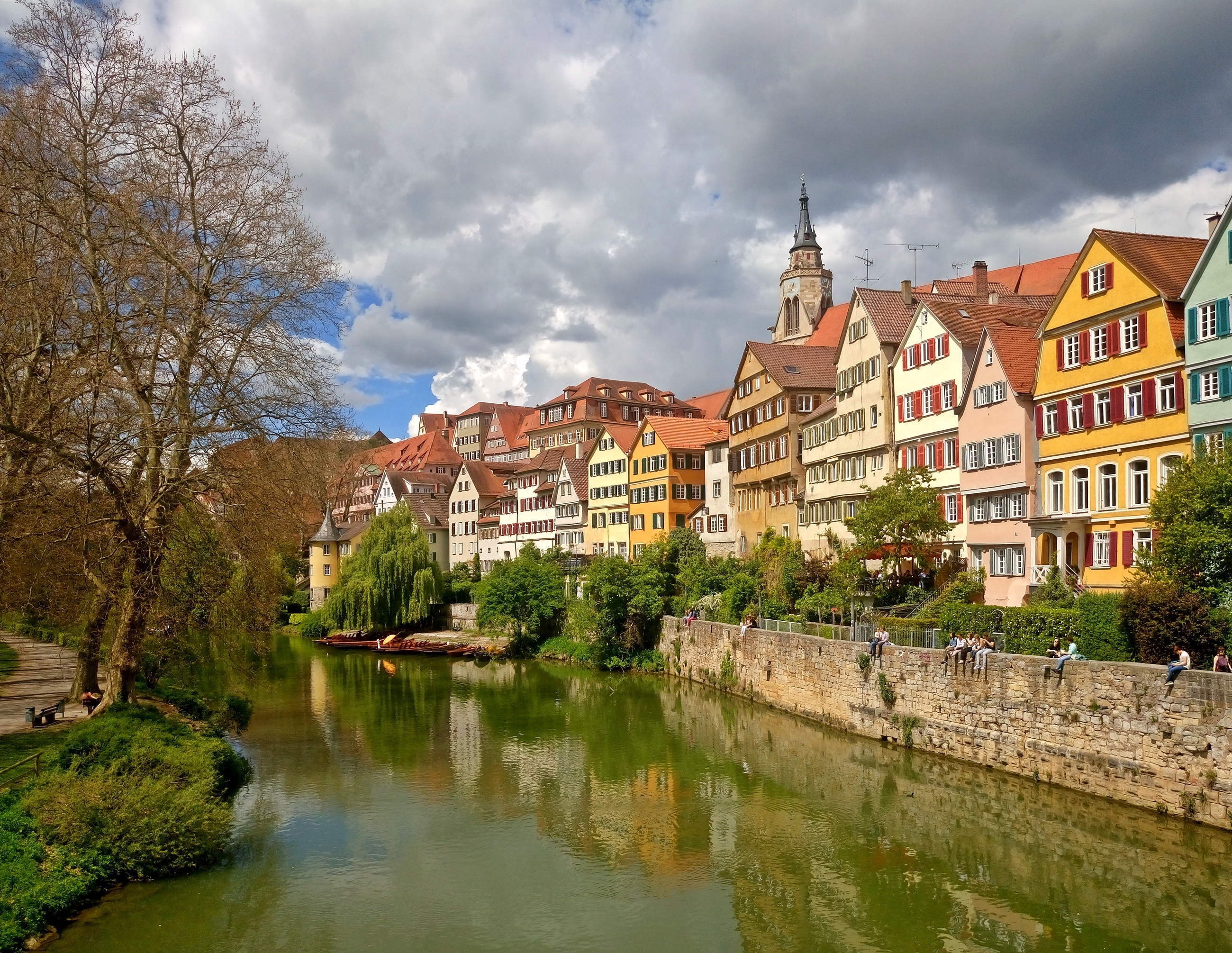
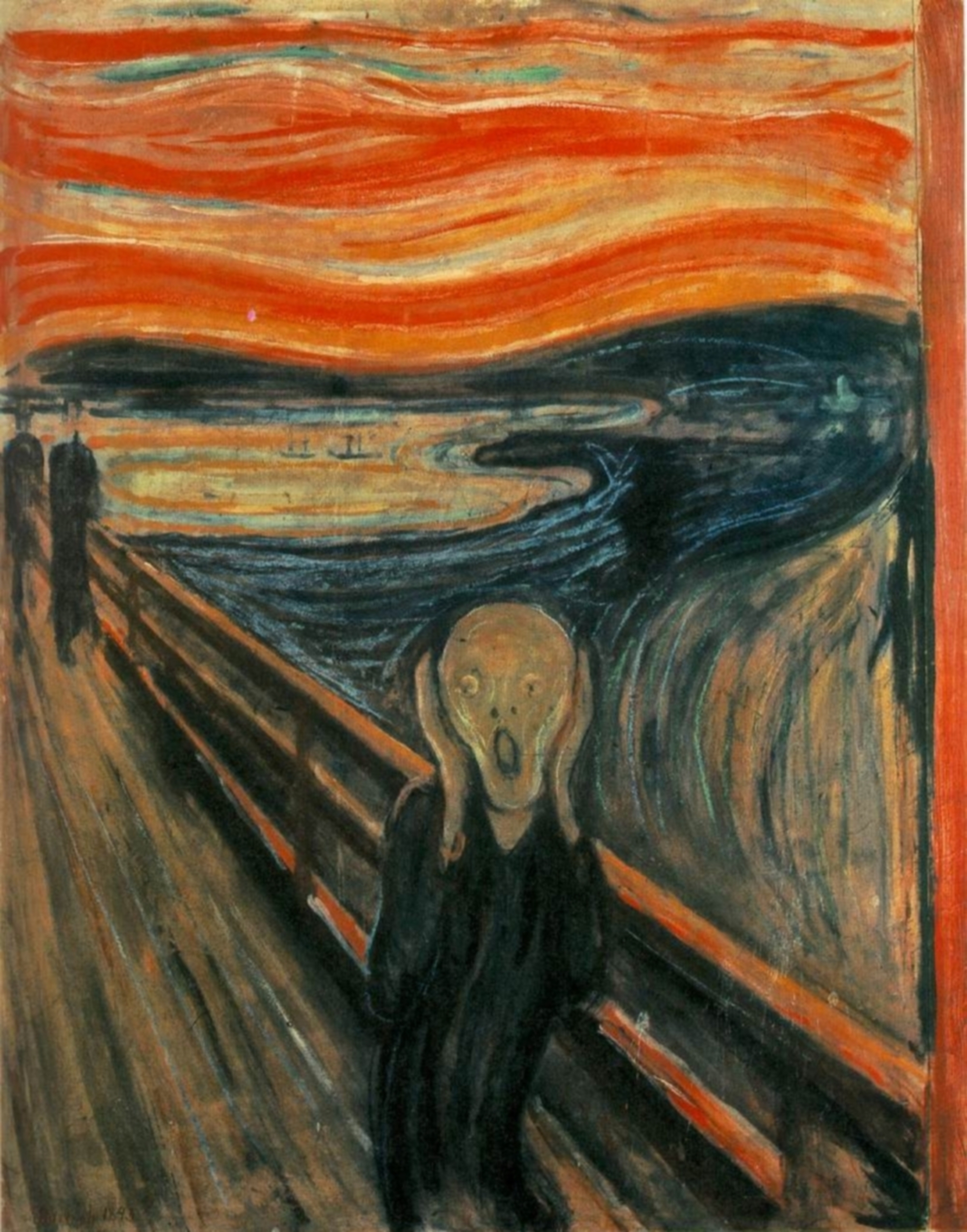
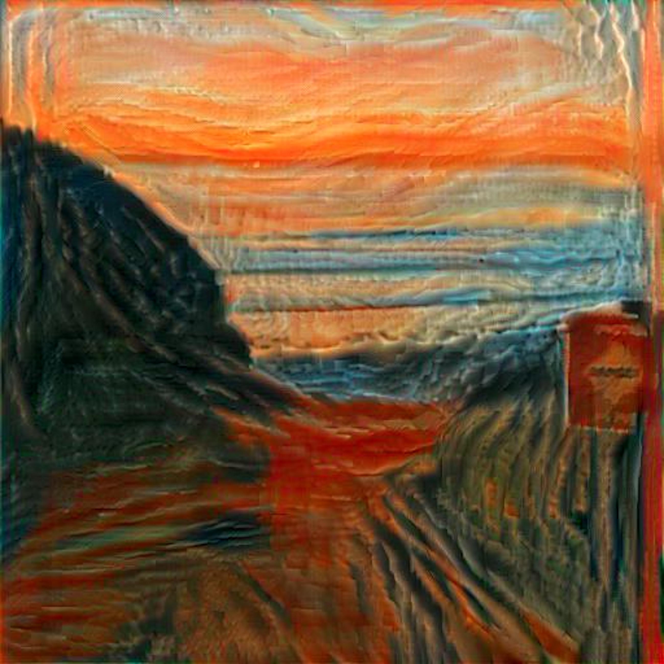
Here is Neckarfront transformed to these three styles:

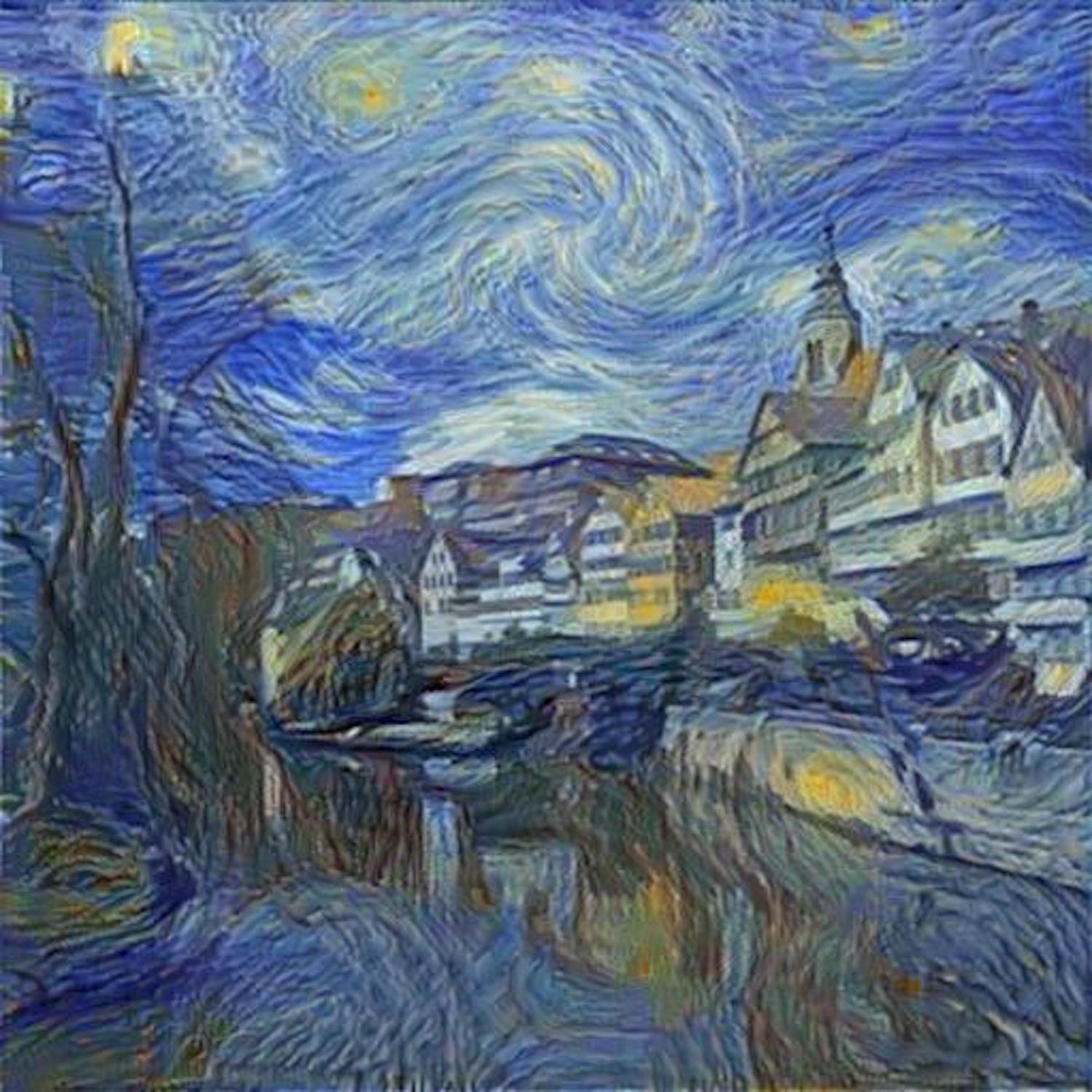
As we can see the results are pretty good although they are not quite like the ones in the paper. This is probably because the authors in the paper performed their descent optimization in a different way/with different parameters. I personally enjoy my results for some images, for exmaple the picasso style from "Femme Nue Assise" output seems better in my implementation because I maintained the content image more so you can still see the neckarfront clearly. However, if we look at the output of the scream style it seems the paper is better as it is smoother. This could perhaps be because of the loss function used. Ideally I would like to use an l1 loss earlier in the network and an mse loss later in the network.

Applying my own styles to Neckarfront + my own images

These are my own images and styles (other than some from above) that I have applied this implementation to:

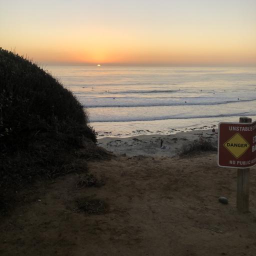
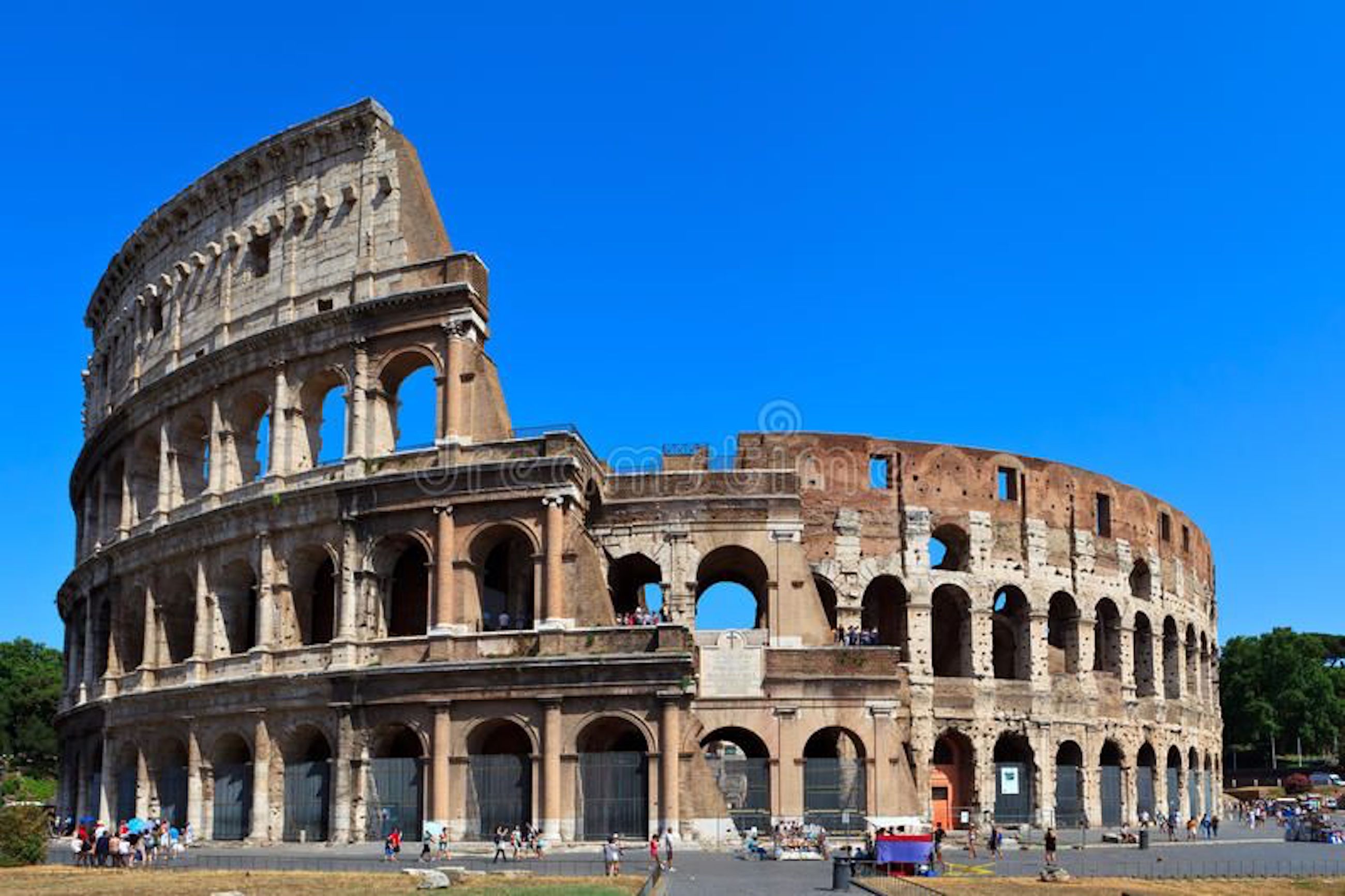
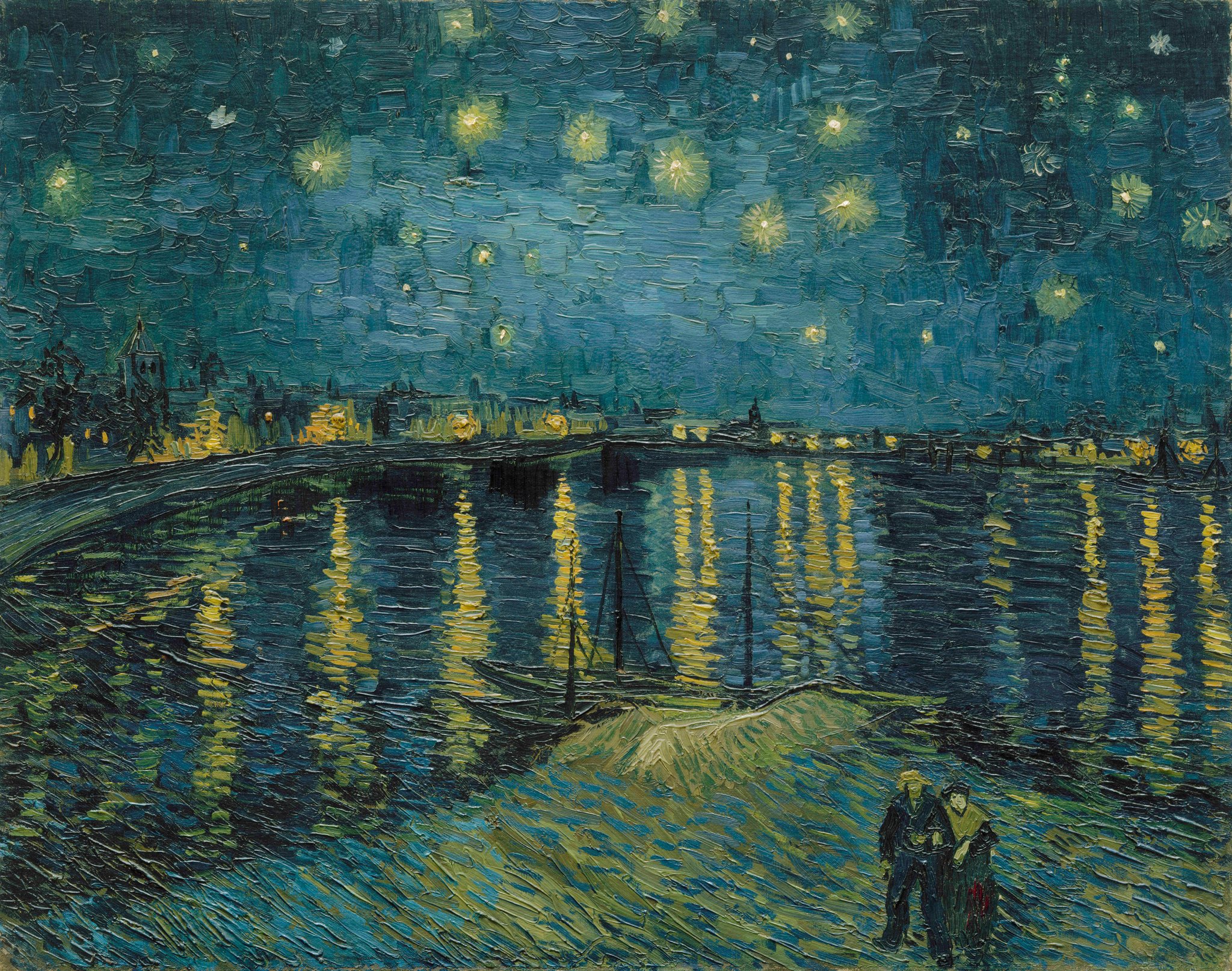
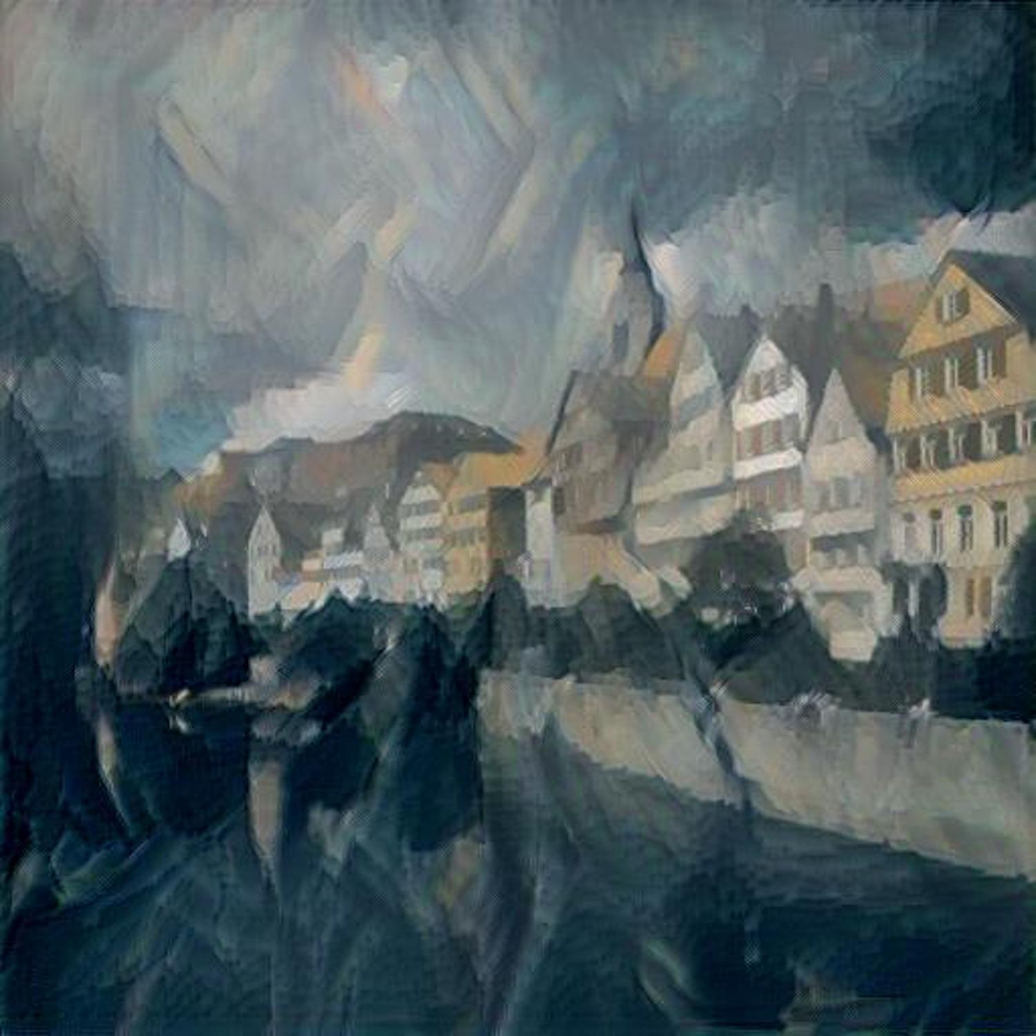
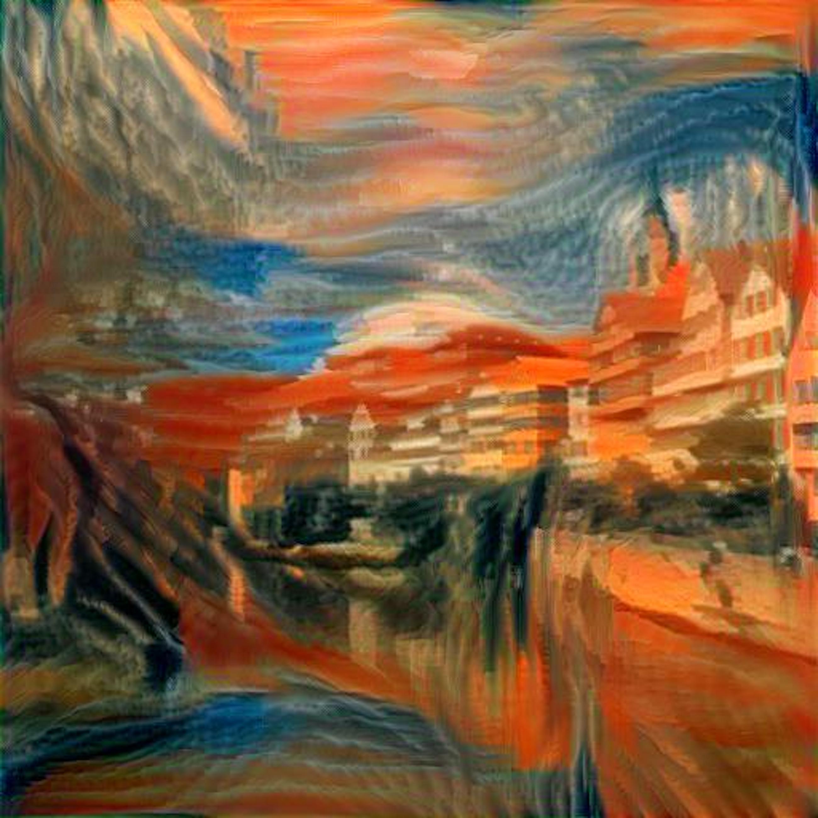
Here is my output, these are outputs that I thought looked really cool and the implementation worked well on:

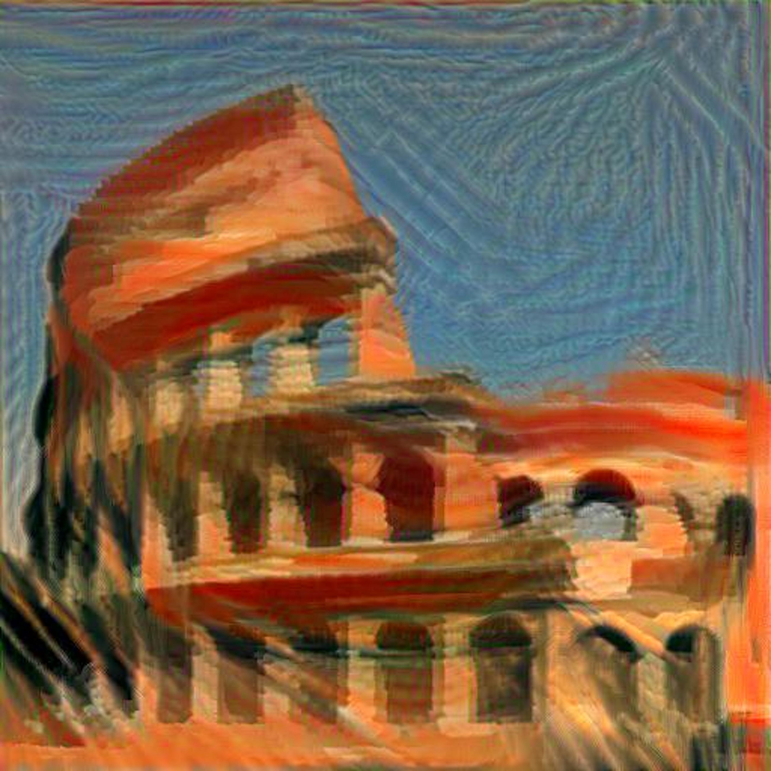
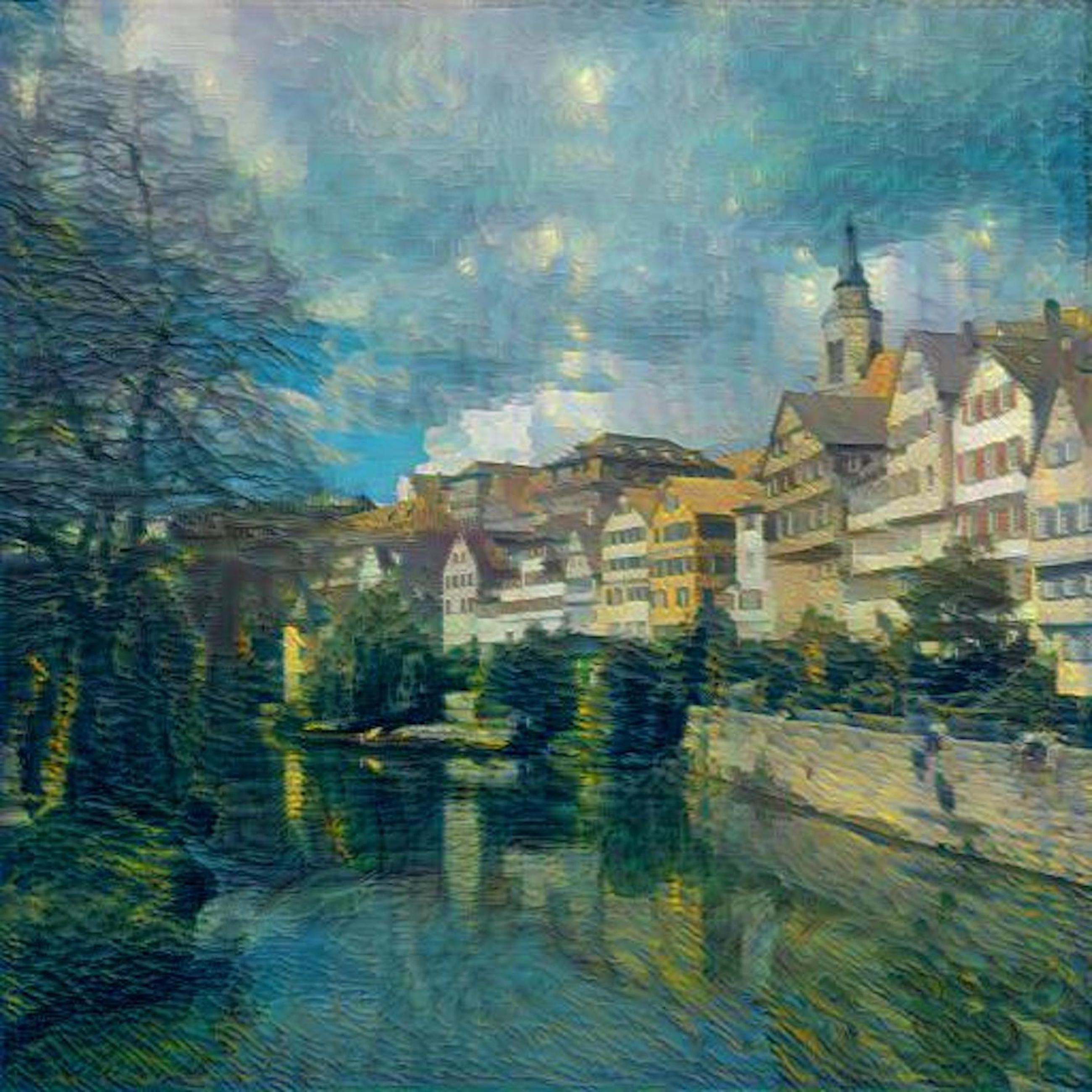
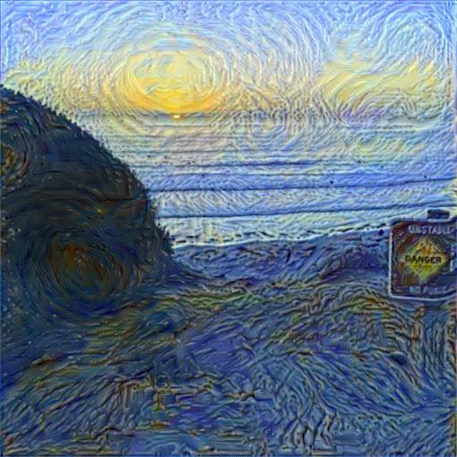
I really like the last one, I had the ratio set to 1e4 and lr = 1e-2, as you can see it still has a lot of the content from neckarfront but it seems like an actual painting by Van Gogh. Here are some results that were pretty bad. I think the reason this was bad is because the original picture had a lot of sunshine in it an starry night style is pretty dark so it had a hard time minimizing the loss function. I tried moving the content loss deeper in the network as the filter reponse at a deeper layer should capture more features of this specific content image. I think the sharp difference between the brightness means it has mostly high frequency components, therefore going deeper should help extract more features of this supposedly "high frequency image". Perhaps the network could be modified to work on this image as well by taking into account that we need deeper cnn layers to extract the high freuency features.

Overall, I thought this was a really fun project and I like the images that came out of it. I think an area of improvement would definitely be to use a different algorithm for gradient descent or even experiment with different loss functions. For example, maybe l1 loss works well with specific styles but not so well with other ones. Another interesting thing owuld be perhaps to have mse loss for the content loss but l1 loss for style loss. I did something similar for the scream neckarfront.

Poor Man's Augmented Reality

Matteo Ciccozzi

For my other final project I decided to implement a Poor Man's Augmented Reality. I really enjoyed the morphing project and the image mosaicing project therefore I decided to meddle with another mapping related project, luckily after project 5 this project was a walk im the park.

Input Videos and Setup

I shot numerous input videos as it was a bit of a trial and error, I realized that the median flow tracker did not work well if we had rapid rotation or large movements. Here you can find all the input videos and output results. Please refer to the first half of the video for inputs and second half for the augmented reality cubes being placed. Click here for the videos.

The first task was to create a box with equally spaced lines to form a grid. This was a necessary step because we need convert 3d coordinates to 2d. For exmaple when we place the cube its verices will be placed at 3d coordinates and having the grid on the box helps us pin point exactly where (1,1,1) maps to for example. I had to create the box twice as the first time the points were too close together, the second box I created is the one used in the videos.

Manually Selecting Points

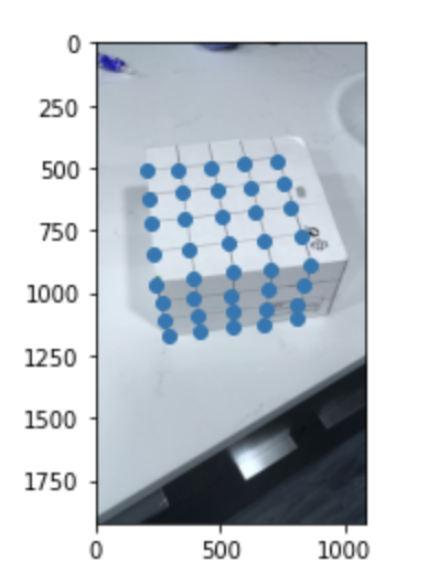
Once the setup was done the next step was to manually select the points of the grid corresponding to integer cooridnates so we could obtain teh actual 2d coordinates in the picture. For exmaple, point (0,0,0), the origin, was chosen to be the bottom left corner of the box and this corresponded to point (518.8, 1802.7) in the actual picture. I used the plt.ginput function to manually label all 40 points. Here is what the manually labeled poitns look like:

Setting up a Tracker

Needless to say, manually labeling all 40 points for each frame would take too long. As a result I used the opencv Median Flow tracker. I initialized it with the first image and the tracked points and just stepped through each frame. The output was pretty good, the tracker kept track of most of the points with very few, and occasional, failures. I experimented with the MIL tracker and the CSRT tracker, however neither of these two achieved the speed and accuracy of the Median Flow tracker.

Calibrating the Camera

As I mentioned, in this project we want to map the virtual coordinates of the cube to physical coordinates in the picture. To do so we need to find the mapping for each point. We know the transformation matrix (calibration matrix) is made up of a 3x3 rotation matrix with an affine translation vector appended at the end. Consequently we have 12 unknowns since the matrix is 3x4. However, as with the previous projects, we actually want the very last entry (bottom right) to be fixed to 1 as we don't want to scale along the virtual z axis. As a result, we only have 11 unknowns. We can set up a system of equation similar to that shown in the lecture "Multiview Geometry: Stereo & Structure from Motion" with the minor difference that our b vector will not be zero. This is done to account fo rthe fact that one of the entries is fixed to one, in fact b will simply be equal to the last column of the matrix shown in lecture. I then use least squares to solve for the optimal vector which I append 1 to and then reshape to be 4x3. I had tried experimenting with the svd and solving the same matrix shown in lecture and then normalizing the last enntry to be 1 however this did not work as well.

Using this method I compute the calibration matrix for each frame's tracked points.

Setting up the Cube Coordinates

At this stage everything is set, all that is left to complete is simply determine where to place the cube! I decided to place the cube such that the bottom left corner of it would be at the virtual coordinates (1,1,3). The box surface was at a height of 3 on the z axis. After this, we can construct a matrix by concatenting all the virtual coordinate column vectors and appending a row of 1 and then transposing everything, at this stage our 4d coordinate matrix is of shape 8x4.

Mapping and Drawing the Cube

At this point I used the calibration matrix to map the virtual coordinates to the actual coordinates (making sure to normalize the 3 entry to be 1) for each frame. I then used the open cv functions found in the resource page to draw the cubes. I did modify them a bit to make the lines thicker, as I thought it looked better. Once the drawing was completed for each frame I simply saved the sequence as a file. Click here for the results (remember to checkout the second part of the video).

Final Reflection

This was definitely one of my favorite projects in the course, I had a lot of fun making it but realized that it was really hard to get a good stable cube in the video. This is because of little oscillations I made while filming that may have thrown off the tracker. There is definitely a lot of room for improvement and exploration, eg. placing different geomatrical shapes on the box. One thing that I will definitely look into is figuring out how this is done on apps like snapchat where there is no predrawn 3d mesh. All in all, this is my last project as a Berkeley undergrad... thank you for the wonderful semester.