In this project, I explored gradient-domain processing, a simple technique with a broad set of applications including blending, tone-mapping, and non-photorealistic rendering.
The primary goal of this assignment is to seamlessly blend an object or texture from a source image into a target image, using gradients to blend the images by changing the overall intensity.
Here, starting with the toy problem, I computed the x and y gradients from an image s, then use all the gradients, plus one pixel intensity, to reconstruct an image v.
We denote the intensity of the source image at (x, y) as s(x,y) and the values of the image to solve for as v(x,y). For each pixel, there were two objectives:
1. minimize ( v(x+1,y)-v(x,y) - (s(x+1,y)-s(x,y)) )^2, the x-gradients of v should closely match the x-gradients of s
2. minimize ( v(x,y+1)-v(x,y) - (s(x,y+1)-s(x,y)) )^2, the y-gradients of v should closely match the y-gradients of s
We also have one additional objective to handle that these could be solved while adding any constant value to v:
minimize (v(1,1)-s(1,1))^2, where the top left corners of the two images should be the same color.
I then used least squares as an optimization function to recover the original image. For the least squares formula Ax=b, A's rows correspond to x and y gradients, x is the vectorized pixels, and b is the vector containing the results to the gradient equations.


The result is pretty similar to the original with a little inconsistency of texture and color, probably as a result to not an exactly zero error when calculating least squares.
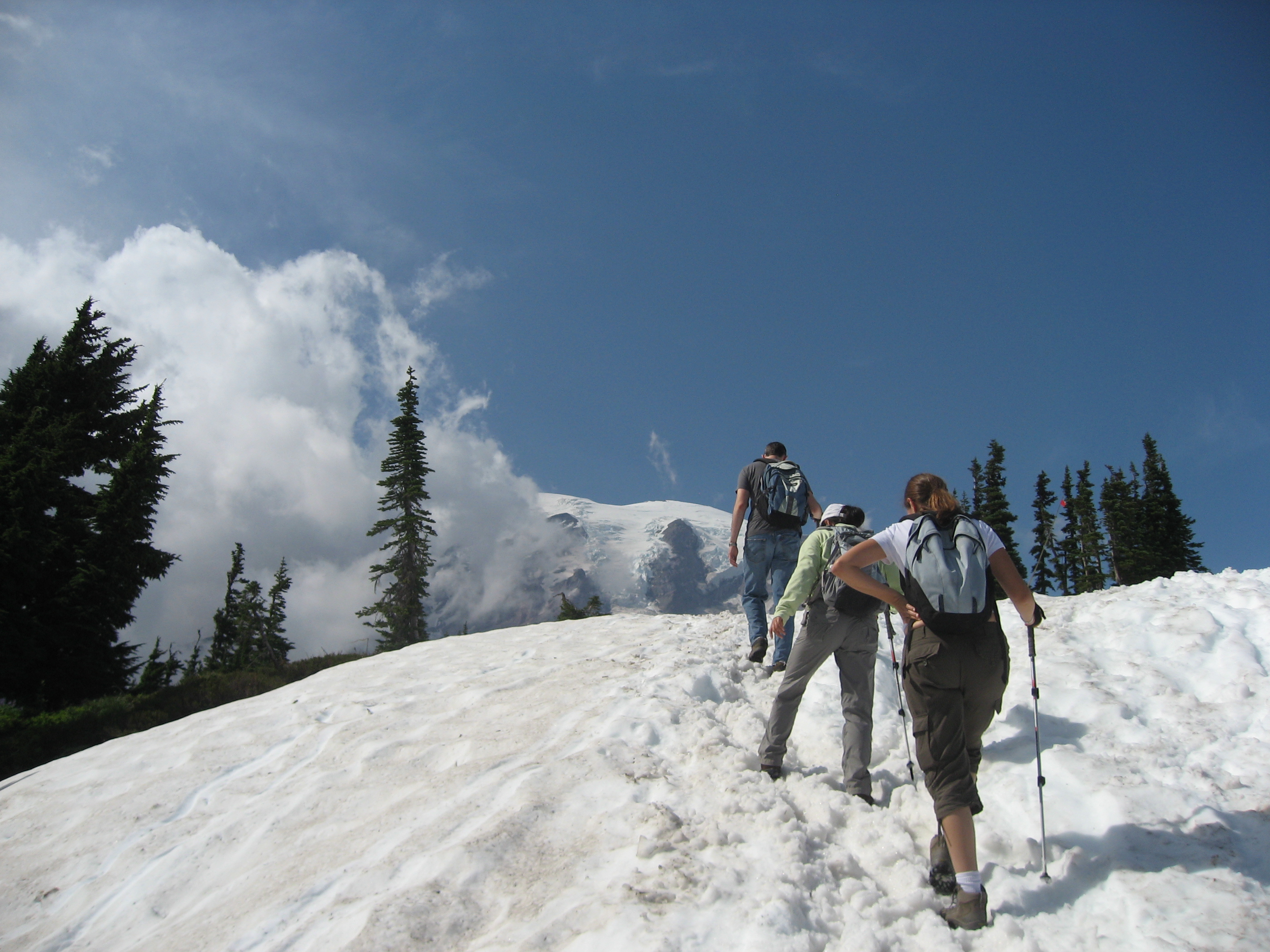
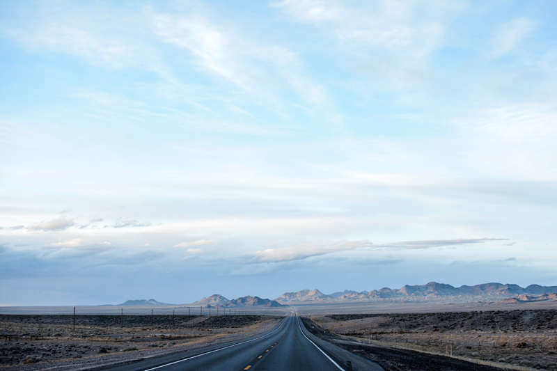
First, I created a bunch of masks for my example source images. I chose images with relatively similar background color as the surrounding area of the target region.
Next, I solved for the blending constraints, using the formula:

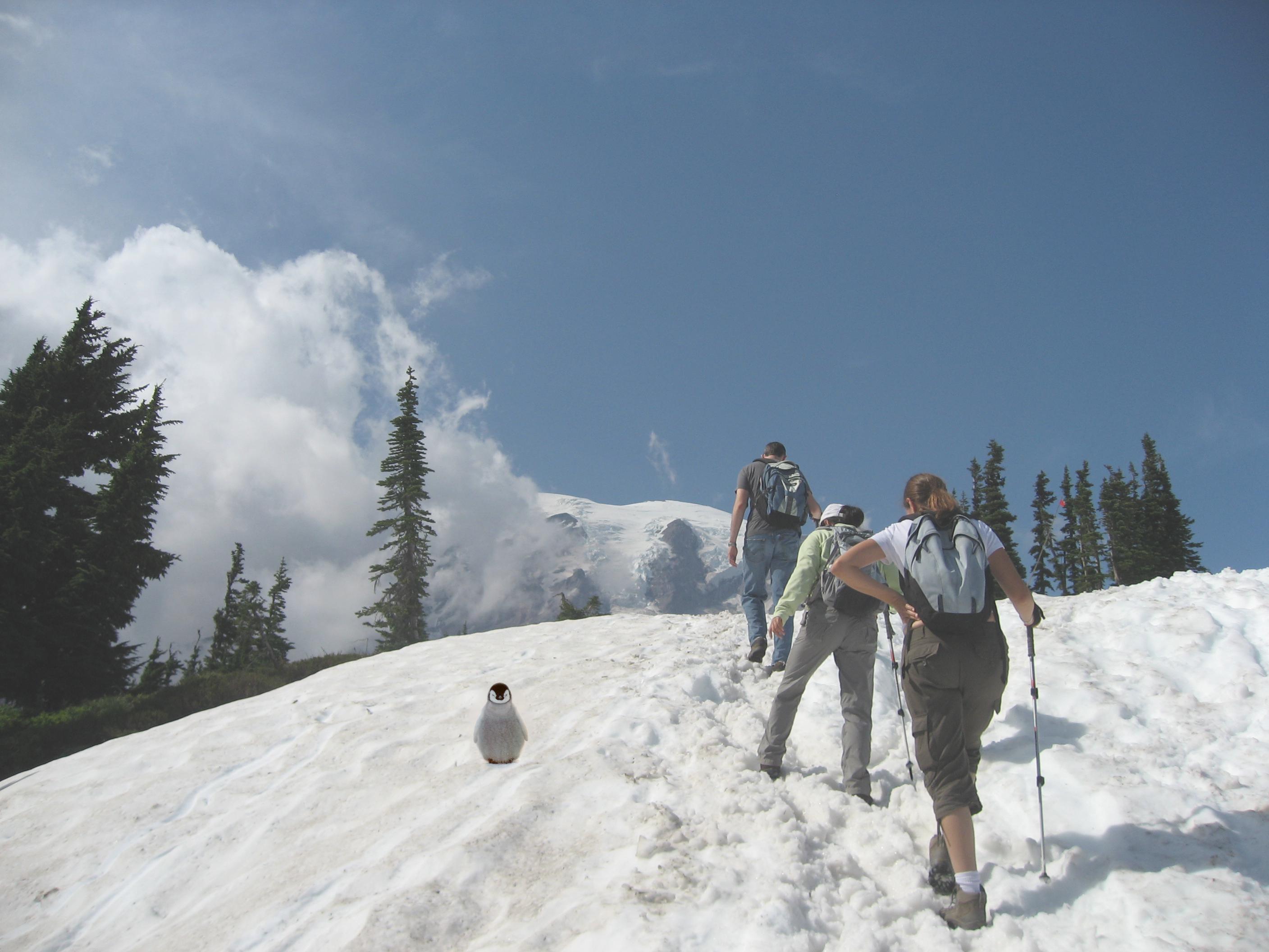
Finally, I copied the solved values v_i into my target image, processing each color channel separately for these colored images.
The overall process was relatively similar to the reconstruction of the toy problem, except for now I added in the vertical and left gradients into my sparse matrix and copied the target gradients into my destination vector b.
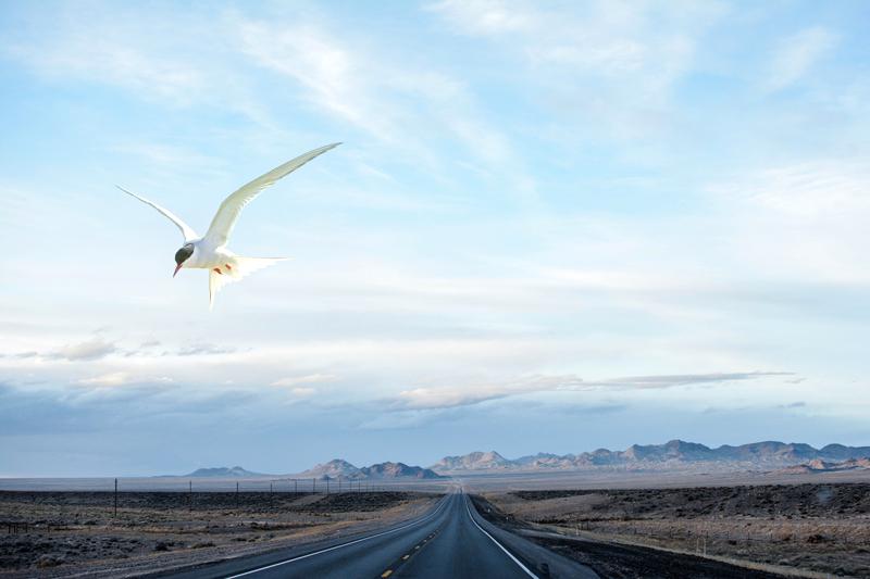
This blend worked relatively nicely because the background of the source image was very similar to the target image, and thus was easy to blend together without looking too jarring. In addition, the textures were similar and there wasn't much variation in color that would cause my poisson process to fail.

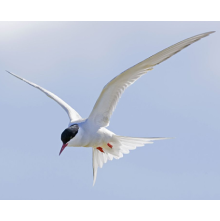
This blend also had a similar result to the first one, as the images complemented each other quite nicely. I think this one especially works because the contrast for the target image was already quite low, making the difference when adding the source image not too jarring.
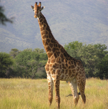
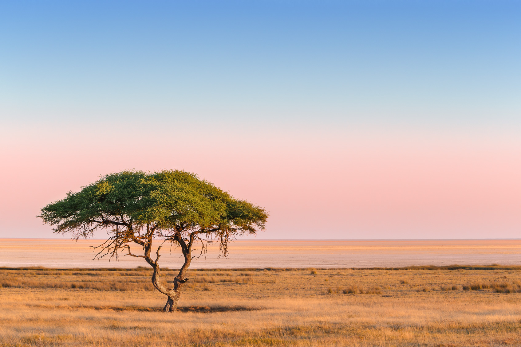
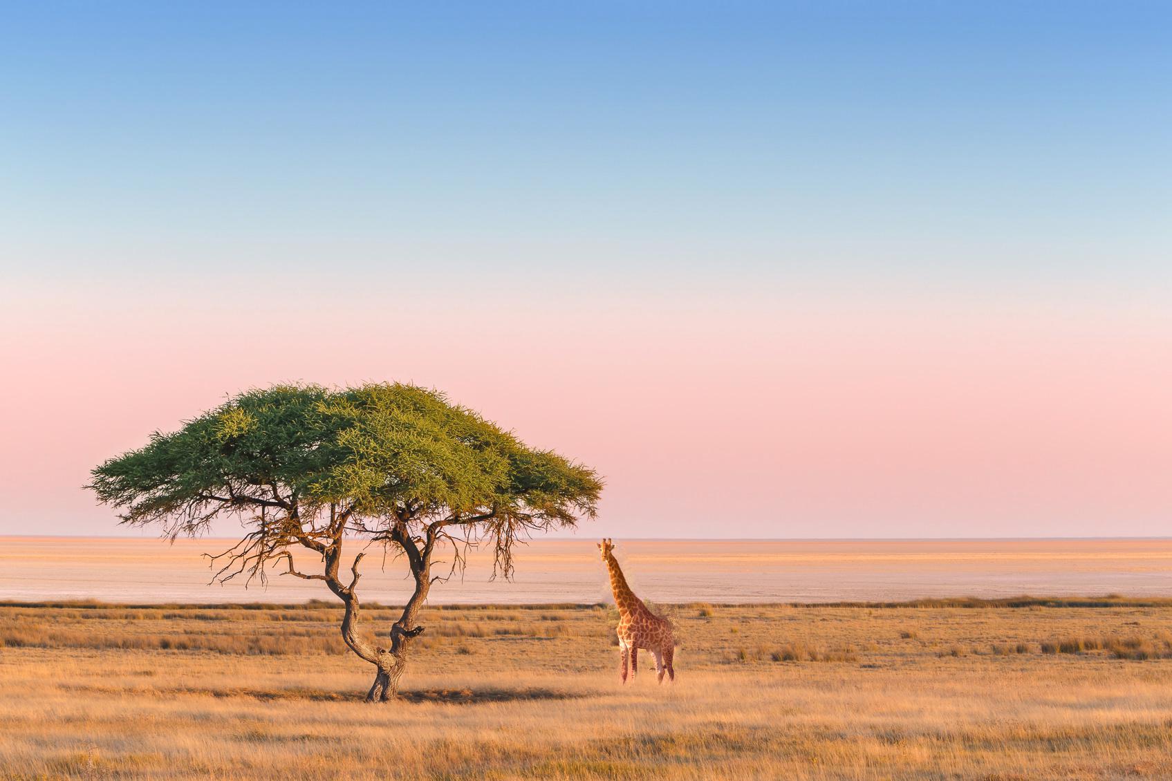
This final blend was not as seamless. This is mostly because the source image I chose had a pretty striking break in the horizon line (it's difficult to find a picture of a giraffe without a break in the horizon line since they are so tall). But because there were trees on the bottom half of the source image, this color and texture was a little harder to blend seamlessly into the target image. The target image is also high in contrast and really sharp, making gradient blending more obvious.
Overall, this part of the project taught me how to use gradient fusion in order to blend an image into another image. I found it interesting to learn the background behind the functions like blend of visualization programs like Photoshop. I also found it cool that this was solved using a simple linear squares function.
In this project, I reproduce depth refocusing and aperature adjustments using real lightfield data.
The main idea of this section comes from the fact that objects which are far away from the camera do not vary their position significantly when the camera moves along one axis direction, while on the other hand, nearby objects do vary. As a result, shifting the images and then averaging allows one to focus on object at different depths.
In this section, I shifted the alpha from 0 to 5, in order to capture the image at different depths.
The main idea of this section comes from the fact that averaging a large number of images sampled over the grid perpendicular to the optical axis mimics a camera with a much larger aperture, while on the other hand, averaging fewer images results in an image that mimics a smaller aperture.
This is because adding images from different angles causes an accumulation of rays from one point on the image, which is the same effect as opening up the aperture. As a result, changing the radius incrementally and then averaging allows one to focus on object at different aperatures.
In this section, I shifted the radius from 1 - 9 to capture the images at different aperatures. I slowed this gif down to show detail, so please be patient:)
Overall, this part of project taught me how to mimic the depth and aperature functions of a fancy camera by averaging images taken from different points on the same axis! It was really interesting to see how such simple functions could create varying depth and opening and closing aperature.