
Original Input Images (Left) == Output Image (Right)
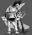
For the final project, I decided to implement Gradient Domain Fusion and Lightfields
Gradient Domain Fusion involves blending an object from another image and seamlessly blending into another image with similar texture and color. This is essentially done by computing masks for our source and target images, which isolate the areas we want to blend. Then we can pick values that closely match the source gradients and blend with the outer boundary of the target region.
The implementation of gradient domain fusion can be complicated because it is neccessary to decompose our objective function into a form that can be solved using least squares. For the toy problem, we are simply reconstructing the provided image, calculating the A and b matrices for the least squares problem, and solving for the output image. This image should match the output image since our source and target here are the same. In order to do this, we must generate the A and b matrix. If N is the # of pixels to be found, then A has 2N + 1 equations where the first N are the 'x' gradients, the next N formulate the 'y' gradients, and the final equation makes sure the top left corner of source and output are same. Using a built in least squares solver, we can find the 'x' vector and reshape to reconstruct the original photo. Below we can see that the input and output images are the same.
Original Input Images (Left) == Output Image (Right)
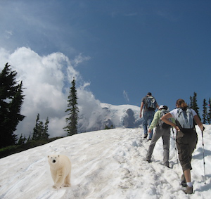
Now that we have some intuition on how to translate our optimization function into a least squares problem, we can implement full blown poisson blending on color images. Poisson Blending is a multi step process that involves extracting a source region from a source image, translating it to the target region of the target image and then performing a blend based on minimizing the optimization equation from the Toy Problem.
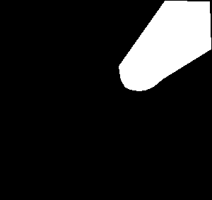
In order to generate the masks, I realized that the provided code was for Matlab which I have no prior experience with. I tried to replicate the tool in python but I was unsuccessful. I decided to leverage Nikhil Ushinde's mask generating code, which was provided earlier by the course. I altered the mask generating code to account for image translation. The code would essentially draw, resize, and generate the masks for the source and target images.
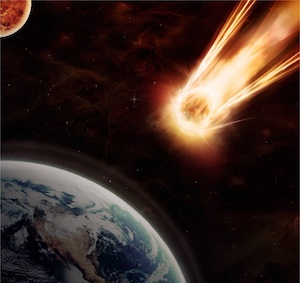
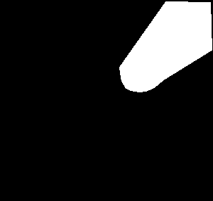
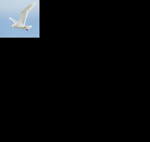
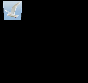
Note the Masks look identical but are actually slightly different. Coincidentally the placement of the comet in source is where I wanted it in the target.
Using our masked source and target images, we can generate the A and b matrix and vecotor. Similiar to the toy problem, we must leverage each pixels and y gradients but now we must also consider the boundaries of each region. We solve for each color channel value seperately. For A, we now have N equations for solving N pixel values. We must consider 4 neighbors for each pixel in the interested region. If the pixel is in the interested region and not on the border, then we account for all 4 neighboring pixels and set the corresponding row in 'b' to be the sum of the differences between the current pixel with the four neighbors. If the current pixel is on the border, then we know at least one of its neighbors is not in the interested region and thus for that out-of-bounds pixel, we use its value in the target image. In the b vecotor, we must now account for the the target pixel value as well as the difference between the source pixels as before. Now we solve for 'x' using least squares.
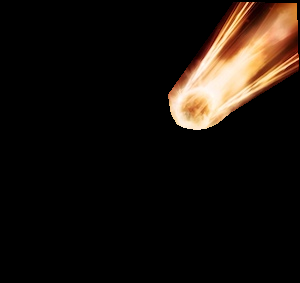
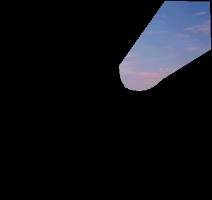
For each of the images, here are the order of the photos shown: source image, source mask, target image, target mask, final blended image

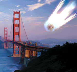
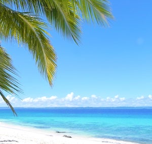
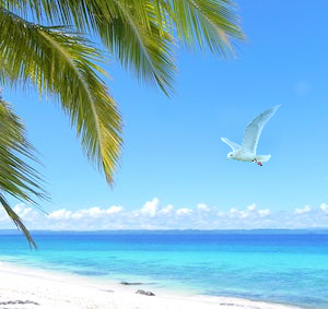
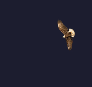
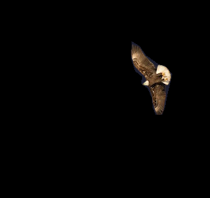
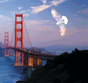
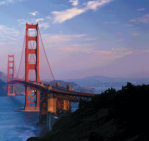
As you can see, the bald eagle in the blended picture is too bright. This failure is most likely due to the stark difference in the background color betweeen the eagle's source image and the golden gate target image. In order to compensate for this drastic difference in gradient in source and target, the error propogates throughout the source region making it much brigher as a whole.
This project was extremely interesting because for the first time in the class, I was finally able to implement effective image blending. The guassian and laplacian pyramid blending of project 2 is not as effective in these cases.
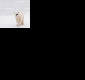
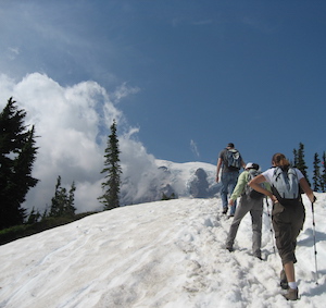
For this project, we tried to implement depth refocusing and aperture adjustment by translating and averaging a grid of pictures taken from my slightly different x,y positions.
In order to get the effect of depth refocusing, we can take a grid of pictures taken by translating the camera and then superimpose and average the images at a particular focal point to focus on different areas of an image. If we take all the photos and simply average them, we see that the back portion of the image seems to be in focuse since the camera translations will have more influence on the frontal features while keeping the features in the back in the same position. Using this intuition, we can shift our images by a certain amount and then average them in order to keep keep one portion of the picture stationary while the other features 'move'.
In order to implement this, I first used the provided grid location of each image and calculated its offset from the center image. Then I translated each grid image by its calculated offset scaled by some scaled factor. This scale essentially determines which area of the image will be the focus point. I used the bracelet dataset from Stanford Lighfields project:
Scale Factor Range is from -1 to 4
Using these lightfield images, we can also mimic varying the aperture. As the spec mentions, if we average a large set of images taken perpendicular to the optical axis of the camera, it acts as if we are changing the aperture of the camera.
To implement this, I chose to focus on the back part of the bracelet. I used the central image of the grid as the smallest aperture. For each depth aperture, I increased the radius of images to average around the center image. Here is how the bracelet aperture adjustment looks at various depths:
Overall, I learned a lot about how lightfield cameras can adjust focus and aperture. Seeing the focus change in the gif is almost magical!
I wanted to create my own lightfield image grid dataset. It turned out to be quite a challenging task. I realized that the lego gantry used in the Stanford Lighfield dataset had to be extremely accurate (sub-millimeter precision). I attempted to build my own rudimentary gantry using a tripod, tape measure, and my phone. Here was my setup:
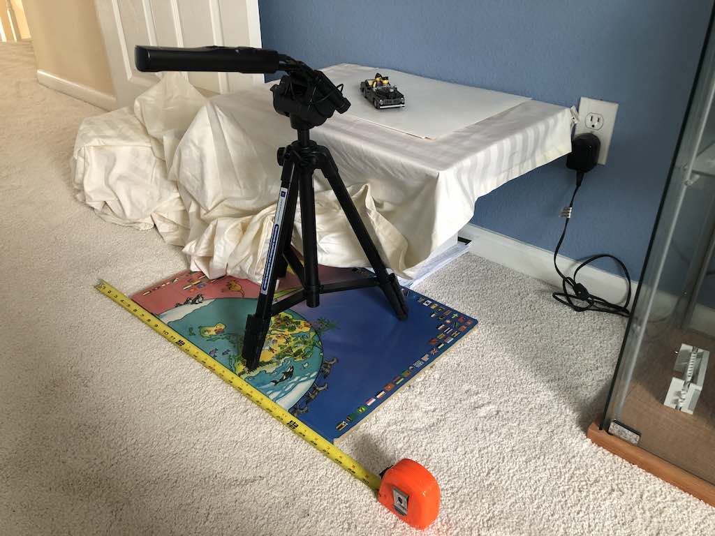
I generated a 5x5 grid of images by translating the x and y direction of the camera by very small amount between photos (~0.15 inch).
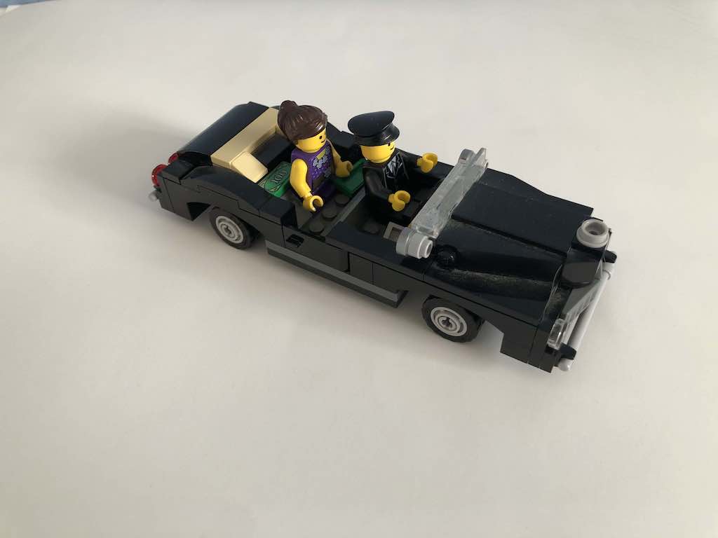

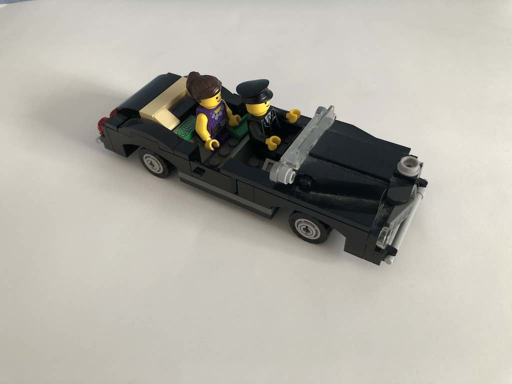
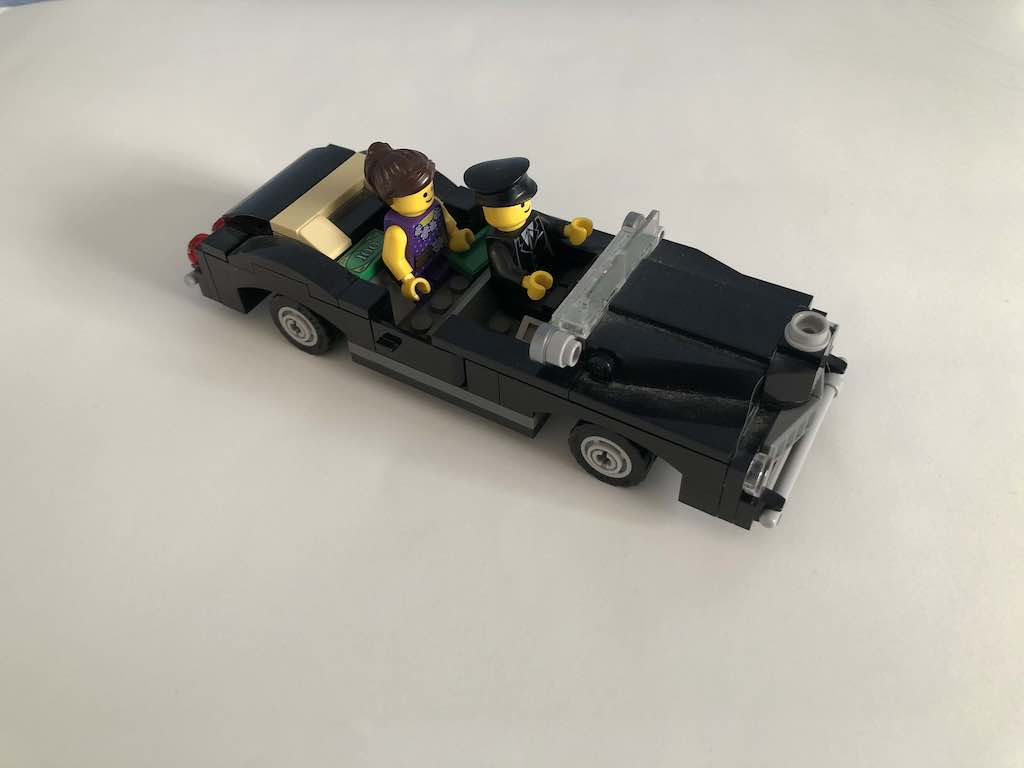

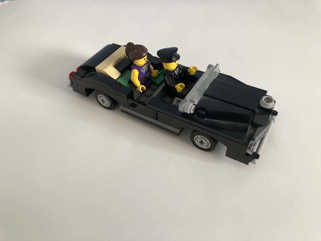

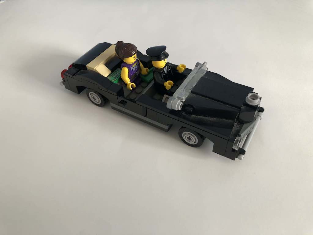
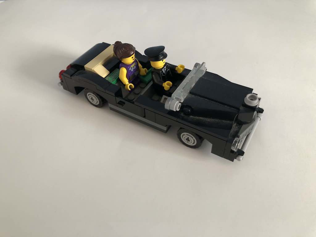
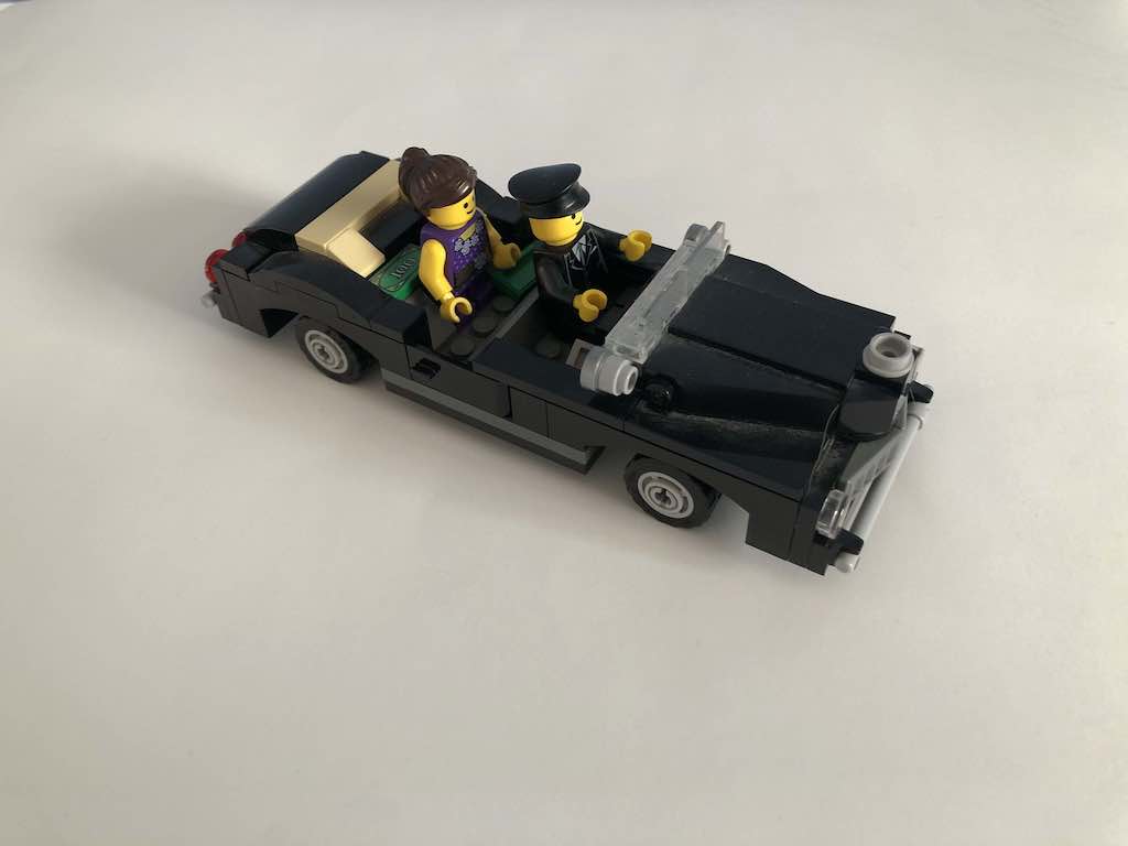
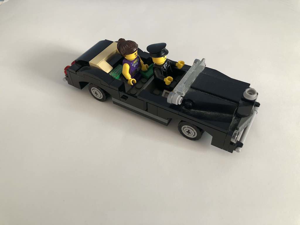


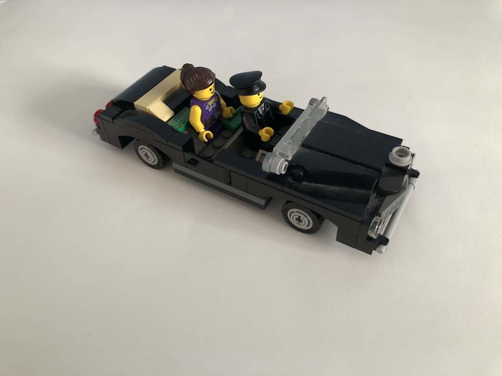


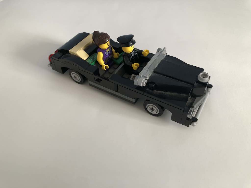
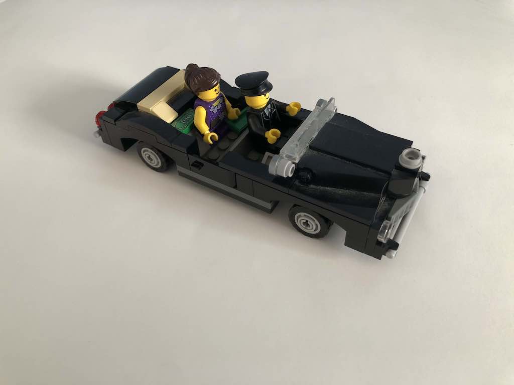
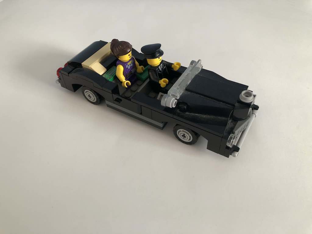
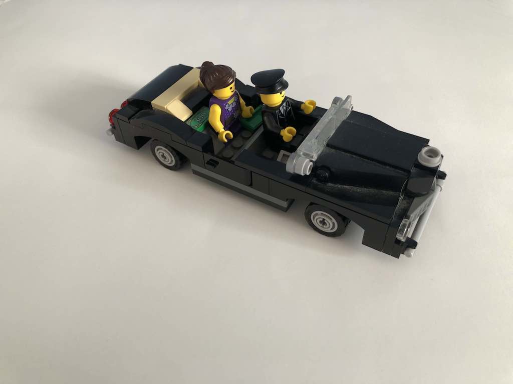
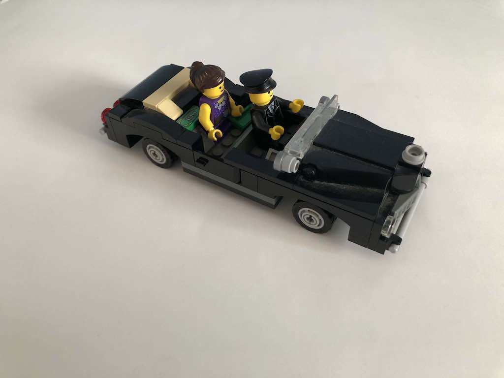

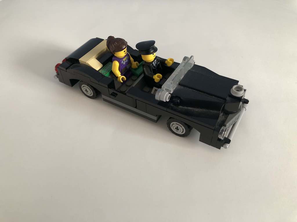
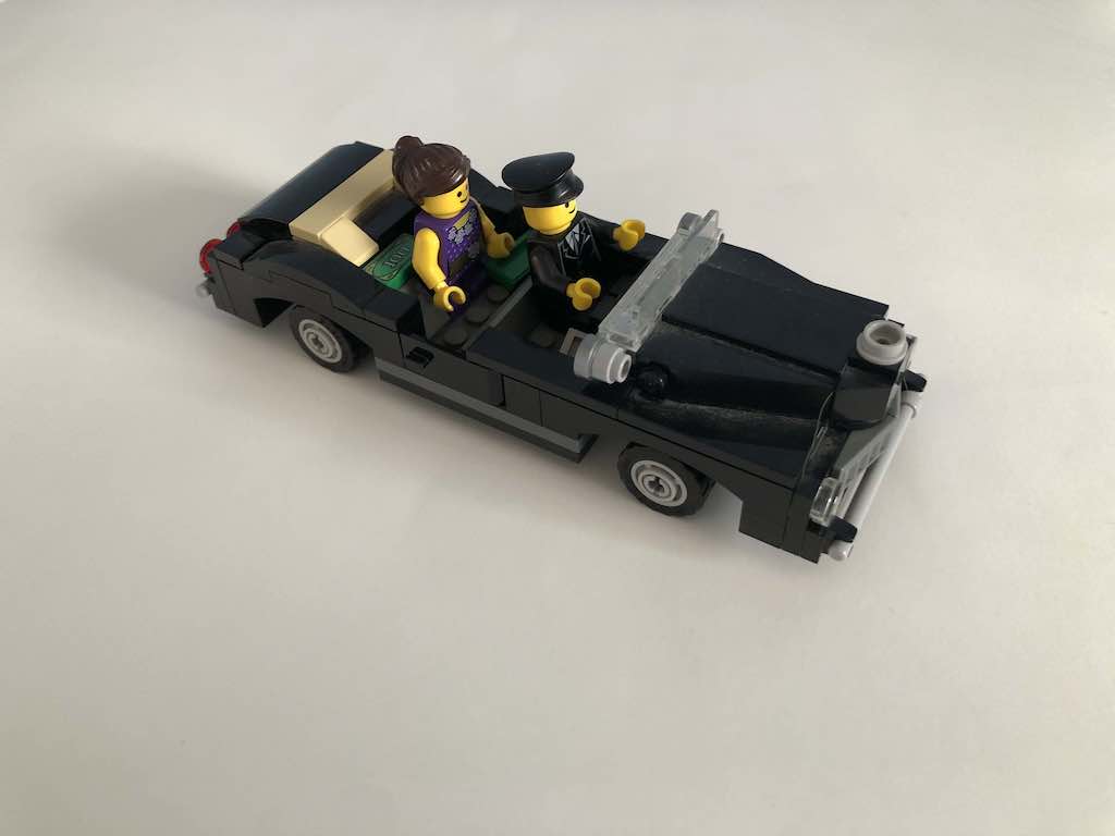
Overall, my attempt was essentially a failure. The image grid produced was not refinded enough and thus the refocusing and aperture adjustments are blurry. I couldn't precisely control the translations between the grid images. I also positioned the car very close to the camera which required my translations to be even smaller between images.