Final Projects
Danji Liu
I picked Light Field Camera and Neural Network Style Transfer as my two final projects.
Light Field Camera
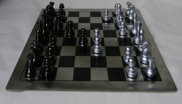
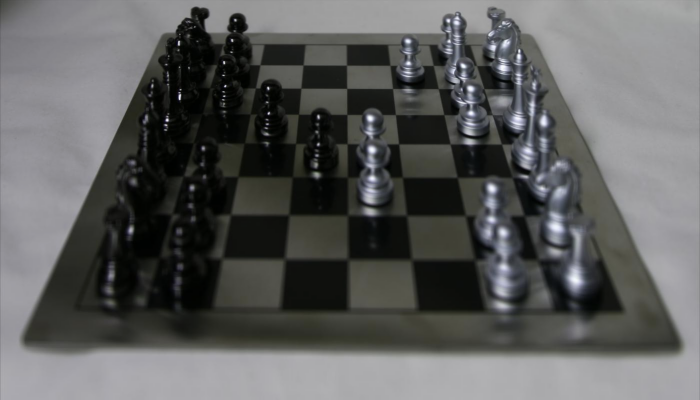
I worked with the images provided at this link. Each light field is represented as a collection of 289 images taken over a 17 x 17 grid. The gird is on a plane that is perpendicular to the optical axis. Each image can be thought of a beam of light that comes through a different part of the aperture. Using the light field camera, we can simulate operations like refocusing or changing the aperture.
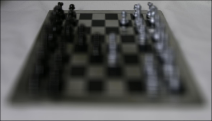
Here are a few examples of the sample images
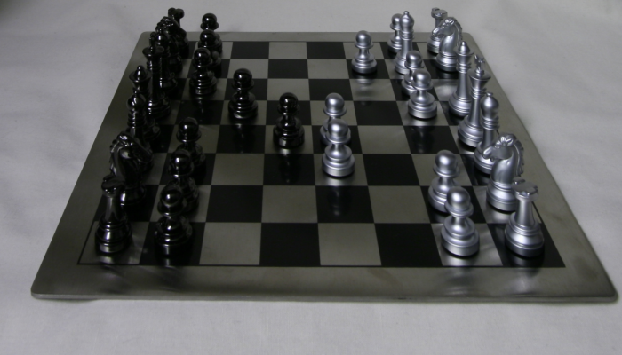
image taken at (0, 0)
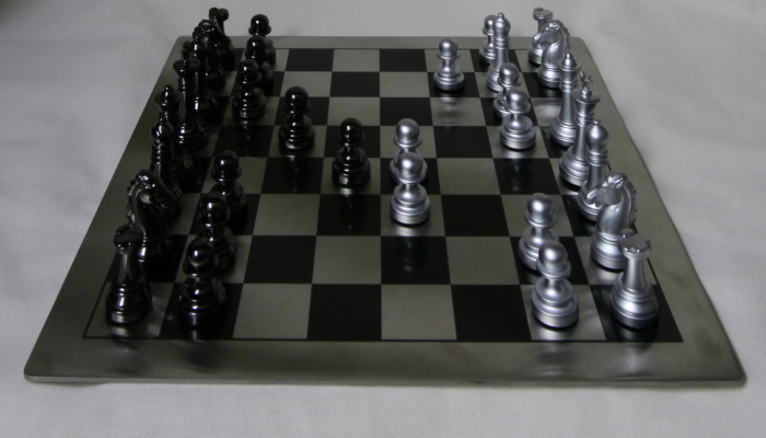
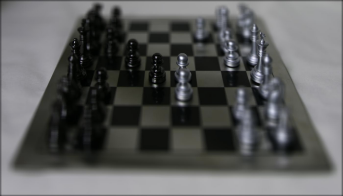
image taken at (8, 8), the center
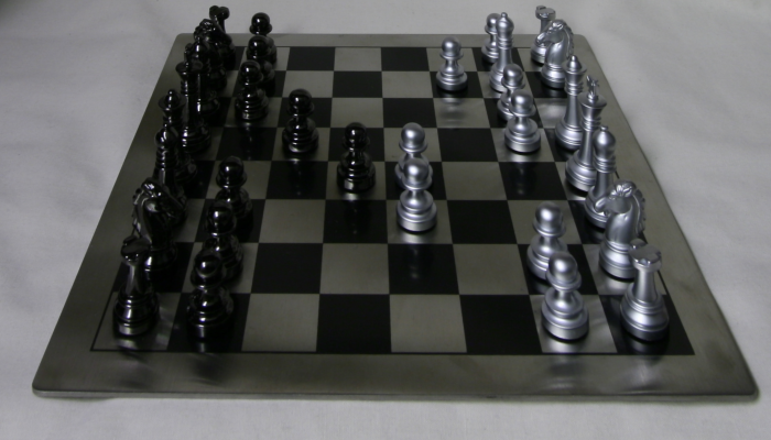
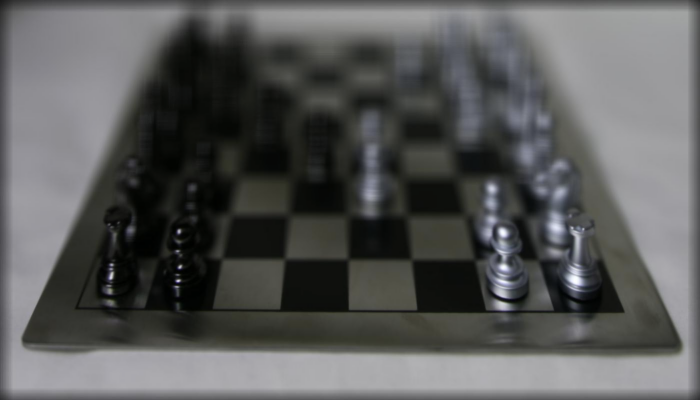
image taken at (15, 4)
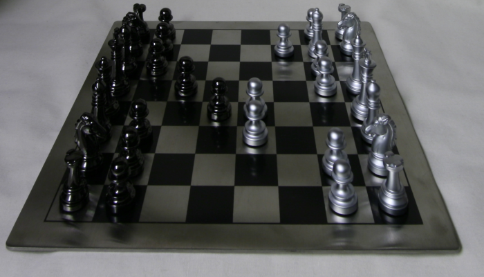
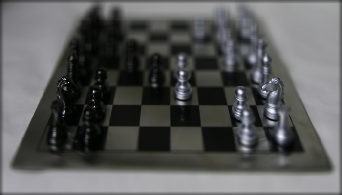
image taken at (16, 16), the last position
Part 1: Refocusing
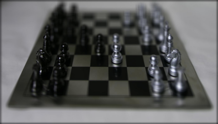
If we average all the images without shifting, the result we get has a focus on the middle of the chessboard. This simulates a regular camera with a certain focal length and aperture.

By shifting the images so that certain features are aligned, we can manipulate the focus of the image and blur other parts of the image. To get the best result, I used all 289 images for refocusing.
The idea is that we shift the images by a certain distance based on the camera positions. The third and fourth numbers of the filename indicate the camera positions u, v. I decide to set the center image at (8,8) to be the base of which all other images shift toward.
Ideally, I would shift the current image by base_u - u horizontally and base_v - v vertically. However, the resulted image looks extremely fuzzy.
The tricky part is to multiply the distance by a scaling factor that's smaller than 1. When the scaling factor is negative, the images will shift away from the center point. Distant objects will become sharp as they are more aligned than close-up objects. On the contrary, when the scaling factor is positive, close-up objects become sharper.
The magnitude of the scaling factor decides how far away the focus is from the original focus in the middle.
scaling factor = -0.2
scaling factor = 0.2
scaling factor = 0.6
scaling factor = 0.4
We can observe the differences of the shifting of focus by changing the scaling factors. The following gif illustrates the process
scaling factor from -0.4 to 0.7
Part 2: Aperture Adjustment
The more images we average over, the more light go through the camera lens. The number of images simulates the aperture size. By selecting fewer images, we can imitate the effect of a smaller aperture. Likewise, more images will simulate a larger aperture.
I approached this problem by picking the pictures within a range around the center image at (8,8). When the radius of the box is 0, the only source image is just the centered image itself. When the radius of the box is 1, I average over a 3x3 grid of images around (8,8), ultimately performing the same procedure in part one but with fewer samples. Finally, when the box radius is 8, I use all of the 289 images.
Since we're only changing the aperture, I picked a fixed focal length by setting the scaling factor to a fixed value. In this section, I set it to 0.1 because the center is on focus.
small aperture. box size = 1 x 1
mid aperture; box size = 7 x 7

mid aperture; box size = 11 x 11

large aperture; box size = 15 x 15
The gif below simulates the process of adjusting apertures by varying the number of image samples.
Bells and Whistles - Interactive Depth Focusing
I used the same method in project 1 to find the best x, y offset. My goal is the find the scaling factor that would give me the best offset for the index-0 image.
Specifically, I look at a 100x100 patch around the selected point to calculate the ssd. On the 0-index image, I walk over a 100 x 100 grid to find the best offsets. For each offset pair, I calculate the ssd of two patches: the patch of the 0-index image and the patch of the target image. After getting the ideal x_offset and y_offset, I proceed to compute the scaling factor using the following formula
scale_y and scale_x will be very close. In the case below when the selected point x = 400 and y = 500, the scale_y is 0.36 while scale_x is 0.35.
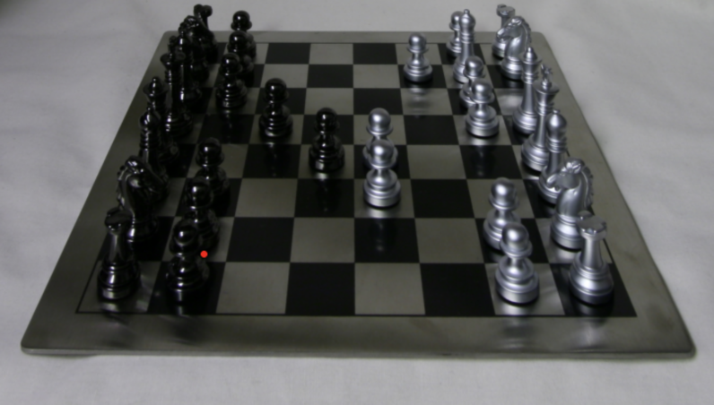
Below is a result of refocusing with a scaling factor of 0.36. Notice the area around the selected point is in the focus while the rest is blurry.
More examples
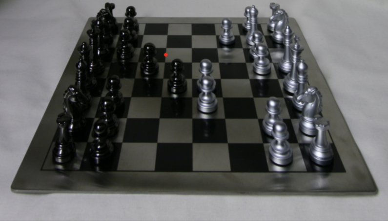
original + selected point
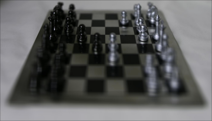
focused. Scaling factor = 0.19
What I learned
Sometimes, a complex problem requires a simple solution. I was surprised that the refocusing is as simple as average over the shifted images.
A few technical problems I encountered during this project
cv2reads the image in the wrong order of channels. It reads in BGR instead of RGB. I had to manually fix the channel order so that nothing weird happens when I display the images usingplt.imshow()
- Again, the rows and cols in image representation is tricky. My translation function (shift) didn't work initially because I mixed up the order
Neural Network Style Transfer
Loader
According to the paper, I used a modified VGG network to train the dataset. VGG networks are trained on images with each channel normalized by mean=[0.485, 0.456, 0.406] and std=[0.229, 0.224, 0.225]. When I load the images into the network, I would call Normalization to convert the data accordingly. I also transform the data whenever I need to get the image pixels from a tensor.
Meanwhile, in my Loader, I also called transforms.Resize, which gives me the flexibility to change data size. I tested my model on smaller data to ensure validity while I used larger data samples to get better-quality results. In most of the runs, I set the height to 512, keeping the images consistent.
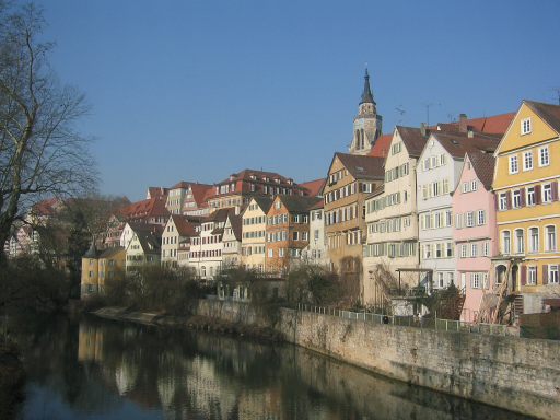
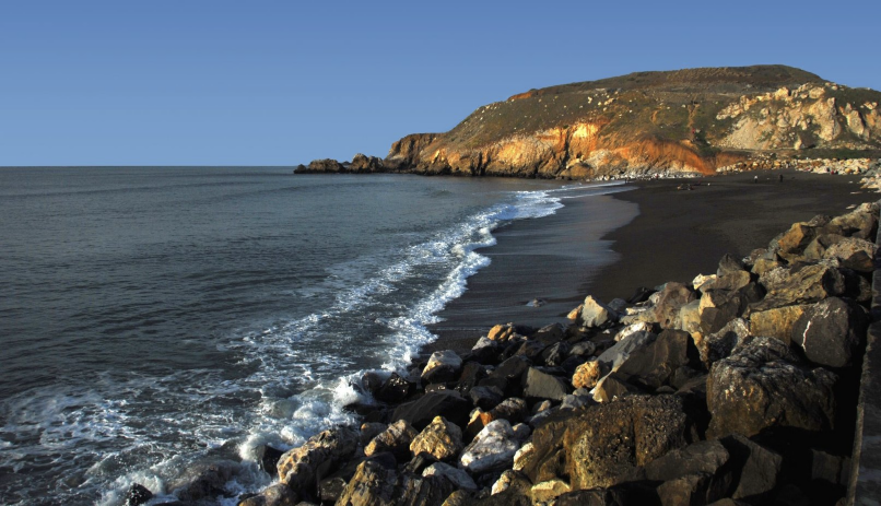
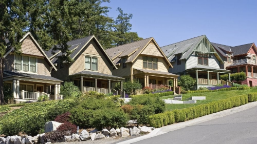
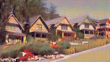
content image
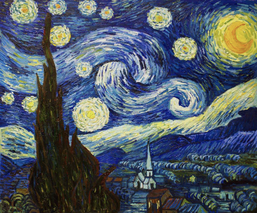
style image
CNN
According to the paper and Piazza, I downloaded a trained VGG model. I reconstruct the image from 6 convolutional layers, 5 of which are style layers and 1 content layer. The layers are conv1_1 , conv2_1 , conv3_1 , conv4_1 , conv4_2 , and conv5_1. I found out the indices related to the convolutional layers in the given vgg model and wrote a get_features function to extract the images of each convolutional layer.
The paper also advises us to use average pooling layers to subsample the features. I enumerated all the layers of the pre-trained vgg network and swapped the max-pooling layers with average-pooling layers of size 2x2 and padding of 2.
I didn't change the size of the convolutional layers of the pre-trained model. However, I clipped all the unnecessary layers after the last ReLU layer at index 29.
The following is the vgg model I used. Unlike the paper, I used fully-connected layers in between my subsampling layers.
Sequential(
  (0): Conv2d(3, 64, kernel_size=(3, 3), stride=(1, 1), padding=(1, 1))
  (1): ReLU(inplace=True)
  (2): Conv2d(64, 64, kernel_size=(3, 3), stride=(1, 1), padding=(1, 1))
  (3): ReLU(inplace=True)
  (4): AvgPool2d(kernel_size=2, stride=2, padding=0)
  (5): Conv2d(64, 128, kernel_size=(3, 3), stride=(1, 1), padding=(1, 1))
  (6): ReLU(inplace=True)
  (7): Conv2d(128, 128, kernel_size=(3, 3), stride=(1, 1), padding=(1, 1))
  (8): ReLU(inplace=True)
  (9): AvgPool2d(kernel_size=2, stride=2, padding=0)
  (10): Conv2d(128, 256, kernel_size=(3, 3), stride=(1, 1), padding=(1, 1))
  (11): ReLU(inplace=True)
  (12): Conv2d(256, 256, kernel_size=(3, 3), stride=(1, 1), padding=(1, 1))
  (13): ReLU(inplace=True)
  (14): Conv2d(256, 256, kernel_size=(3, 3), stride=(1, 1), padding=(1, 1))
  (15): ReLU(inplace=True)
  (16): Conv2d(256, 256, kernel_size=(3, 3), stride=(1, 1), padding=(1, 1))
  (17): ReLU(inplace=True)
  (18): AvgPool2d(kernel_size=2, stride=2, padding=0)
  (19): Conv2d(256, 512, kernel_size=(3, 3), stride=(1, 1), padding=(1, 1))
  (20): ReLU(inplace=True)
  (21): Conv2d(512, 512, kernel_size=(3, 3), stride=(1, 1), padding=(1, 1))
  (22): ReLU(inplace=True)
  (23): Conv2d(512, 512, kernel_size=(3, 3), stride=(1, 1), padding=(1, 1))
  (24): ReLU(inplace=True)
  (25): Conv2d(512, 512, kernel_size=(3, 3), stride=(1, 1), padding=(1, 1))
  (26): ReLU(inplace=True)
  (27): AvgPool2d(kernel_size=2, stride=2, padding=0)
  (28): Conv2d(512, 512, kernel_size=(3, 3), stride=(1, 1), padding=(1, 1))
  (29): ReLU(inplace=True)
)
Loss
For the feature layers (style and content), I calculated the mean-squared distance between the two Gram matrices from original and generated images. The total style loss is the weighted combination of each layer. In the paper, the weights are set to be 0.2 for all five of the style layers. In my practice, I set the first weight to be 0.5 while the rest to be 0.2.
When combining style and content losses, the paper advises us to use a ratio where alpha is the weight of content loss and beta is the weight of style loss. In my code, I set the ratio to because it gives me the best result. Specifically, alpha is set to 1 whereas beta is .
Optimizer & Results
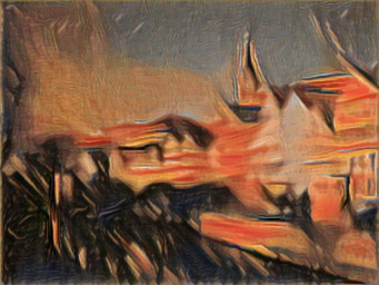
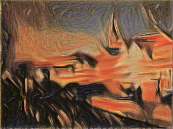
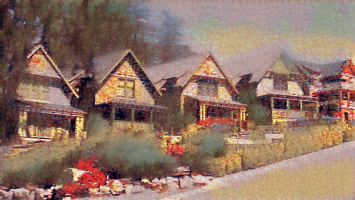
I used the standard Adam optimizer. However, I experimented with many different learning rates to obtain the best result. The following are the image results of different epochs and different learning rates. The best results are when the learning rate is 0.2.
Learning rate = 0.1. Epoch = 1200

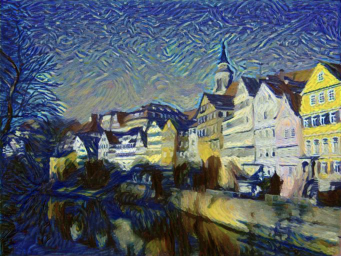
Learning rate = 0.2. Epoch = 1200
Learning rate = 0.4. Epoch = 1200

Learning rate = 0.1; Epoch = 2000
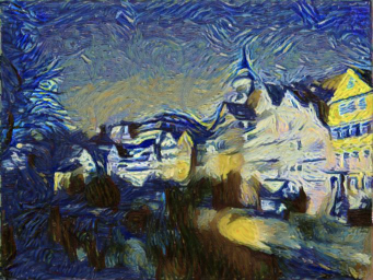
Learning rate = 0.2; Epoch = 2000
Learning rate = 0.4; Epoch = 2000
Compare my results to the paper
As we can see the results closest to the best image is when learning rate = 0.2. The difference between my results and the paper is that mine has more colors from the original content. For example, the pink buildings in the original image are still sort of pink in my image. However, they're all yellow or blue in the paper.
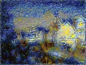
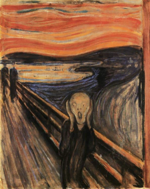
Other styles in the paper
The Scream
Since I got the best results when learning rate = 0.2, I decided to go with that number for the rest of the styles
Learning rate = 0.2. Epoch = 400
Learning rate = 0.2. Epoch = 1200
Learning rate = 0.2. Epoch = 2000
Compare my results to the paper
In the paper, the outlines of the houses are more visible. Here, we can barely tell if the subjects of the photo are houses. It also has to do with the fact that the style image I used is more desaturated than the one used in the paper.
Picasso
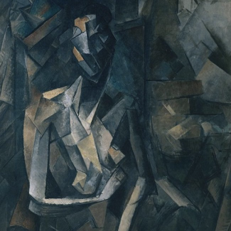
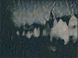
Learning rate = 0.2. Epoch = 400
Learning rate = 0.2. Epoch = 1200
Learning rate = 0.2. Epoch = 2000
Compare my results to the paper
Again, the outlines of the houses in the paper are more visible. The result in the paper has more details at the bottom-left corner of the image. Given that the style image is pretty abstract in the first place, I'm happy with the result.
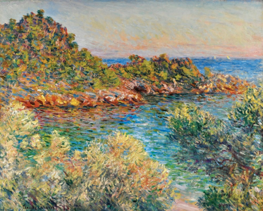
Styles of my own choice
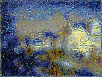
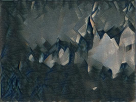
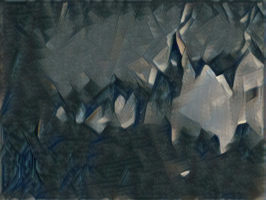
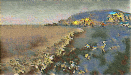
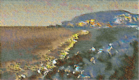
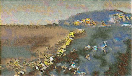
Failed example: Monet
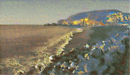
Learning rate = 0.2. Epoch = 400

Learning rate = 0.2. Epoch = 1200
Learning rate = 0.2. Epoch = 2000
Learning rate = 0.3. Epoch = 400
Learning rate = 0.3. Epoch = 1200
Learning rate = 0.3. Epoch = 2000
Why did it fail?
I tried different learning rates but the improvement is minimal. I think the hyper parameters of the network (such as layer size and the number of layers) could be the reason why it failed. The paper didn't use fully-connected layers whereas I did. That could make a big difference. Meanwhile, the beta value (style weight) might be too small.
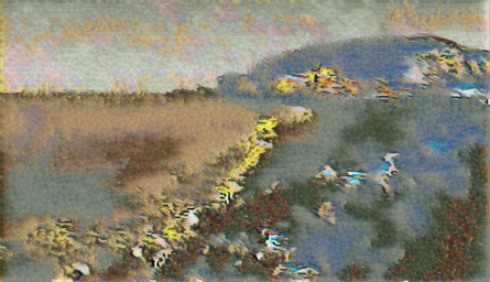
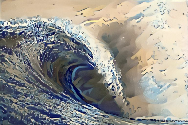
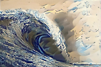
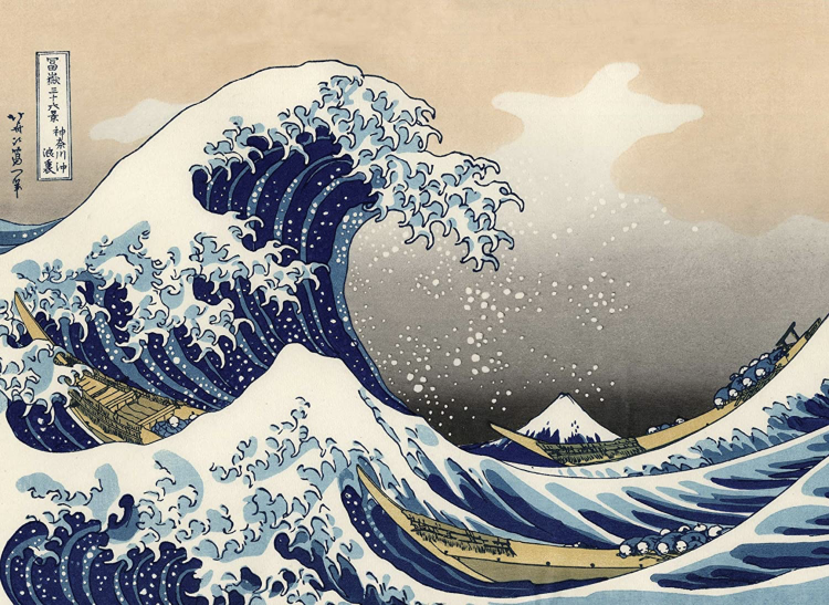
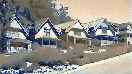
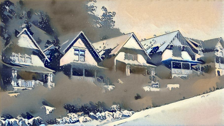
Successful: Waves

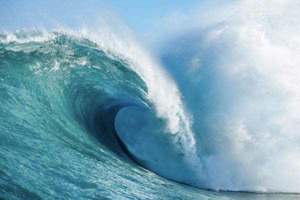
Learning rate = 0.2. Epoch = 400
Learning rate = 0.2. Epoch = 800
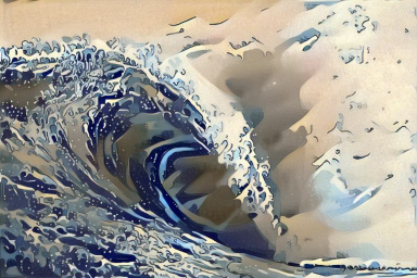
Learning rate = 0.2. Epoch = 1200
Learning rate = 0.2. Epoch = 400
Learning rate = 0.2. Epoch = 800

Learning rate = 0.2. Epoch = 1200
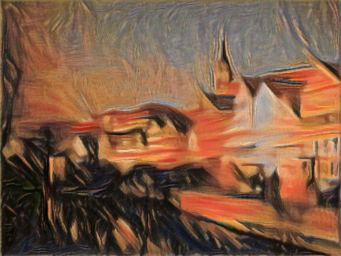
Successful: Fall
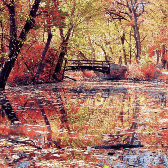
Learning rate = 0.2. Epoch = 400
Learning rate = 0.2. Epoch = 800
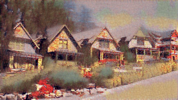
Learning rate = 0.2. Epoch = 1200