Final Project
Vanessa Lin
Image Quilting
Overview
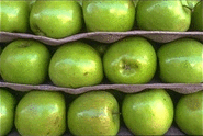
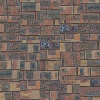
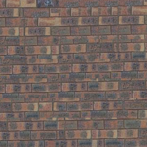
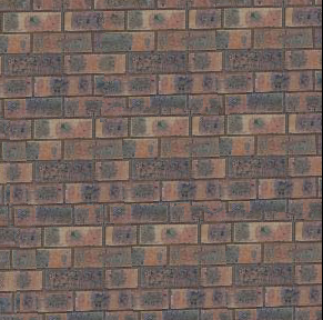
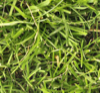
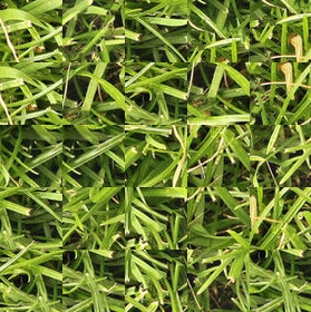
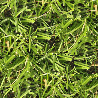
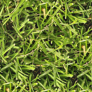
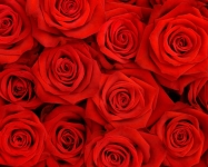
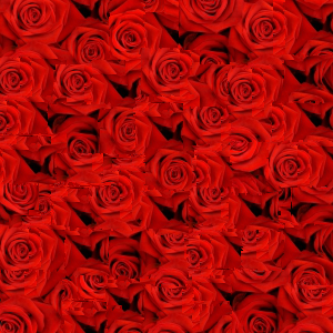
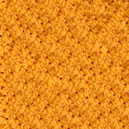
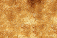
In this project, I implemented image quilting algorithms for texture synthesis and transfer in the SIGGRAPH 2001 paper (Image Quilting for Texture Synthesis and Transfer) by our one and only Professor Efros and William T Freeman. Through these algorithms, I could create larger texture images based on a small sample image and I could transfer texture from one image to another. Below are some sample textures that I used. For the next few sections, I will explain how each texture synthesis process differs and their results through theapples.png texture.
Randomly Sampled Texture
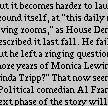
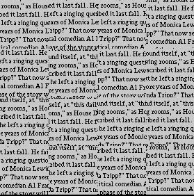
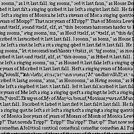
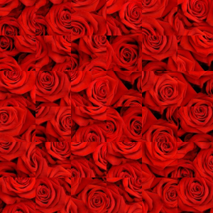
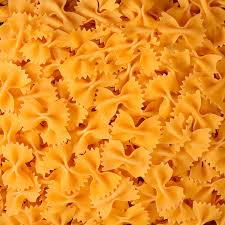
For this method, we fill the blank output image with randomly sampled square patches from the source texture. As you can see below, the edges of the random patches are noticeable and does not look like a cohesive texture.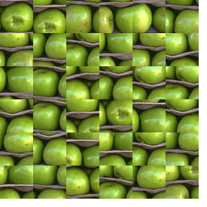
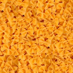
Overlapping Patches
For this method, we start off with a randomly sampled patch on the upper-left corner in the output image and then start overlapping neighboring horizontally and vertically that have low Sum of Squared Differences (SSD) in the overlapped part. For the first row, we compare the neighboring patches horizontally and for the first column, we compare the neighboring patches vertically. For the rest of the rows, we compare the new patch that we're about to select to the previous patch directly above and previous patch to its left. To choose the best patch to place next to the previous patch, I randomly select a patch, which cost is less than themin_cost * (1 + tol), where min_cost is the minimum SSD cost overlap of all the possible patches in the sample texture and 
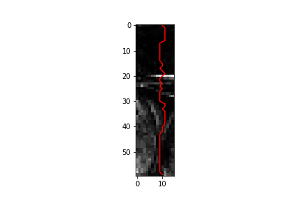
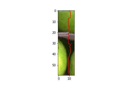
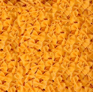
Seam Finding
Building off the Overlapping Patches method above, we find the minimum contiguous path of the overlap between the patch we selected and the previous patch, through computing the cumulative minimum error like socum_E[i, j] = ssd_map[i, j] + min(cum_E[i-1, j-1], cum_E[i-1, j], cum_E[i-1, j+1]). After finding the minimum contiguous path, I created a mask (1s for the region to the right of the path and 0s for the region to the left of the path and vice versa for the other overlap) for the overlaps to combine the overlaps to become a seam overlapped image, like shown below for the apple overlap. I created separate functions to find the vertical seam path and horizontal seam path. For the rest of the rows that overlap with a previous upper patch and previous left patch, I combined the masks that I found from the vertical seam path and horizontal seam path to create a nice seamed overlap.


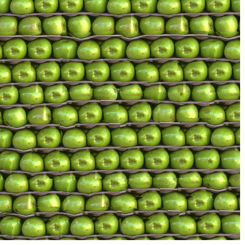
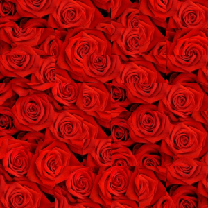
Here is the final result of running the Seam Finding approach on the apples texture. (Now, we have a lot more apples compared to the few that we had originally!)
Results
Here are more results and their progressions through the three different methods that I explained above.
Texture Transfer
For this portion of the project, I applied the texture synthesis technique (Seam Finding Method) to transfer a texture sample to a target image, basically making the target image appear to be that sample while also preserving the general features of the target image. To do this, we redefine our error metric with an extra variable,alpha to be alpha * overlap_ssd + (1-alpha) * corr_ssd , where corr_ssd is the SSD between the correlation map of the target image patch and the sampled texture patch. The correlation map that I used for the texture and target image was image intensities.

Bells and Whistles
For bells and whistles, I created my own version of thecut.m function in Python using dynamic programming, where I find the minimum cost contiguous path horizontally and vertically. In this function, I also returned the mask, where the mask will be all 1s for the region to the right of the minimum contiguous path and all 0s for the region to the left of the minimum contiguous path, for the overlapping images.
What I've learned
I was quite surprised at how well the seam finding method looked on some images, but I think I was more surprised at how well just plain overlapping worked on several images. It was quite cool to implement Professor Efros research paper and I learned a lot more on texture synthesis techniques and how to texture transfer as well. I would like to however better optimize the code in the future, since it takes a while to run on small patch sizes, and create more texture transfer images!Light Field Camera
Overview
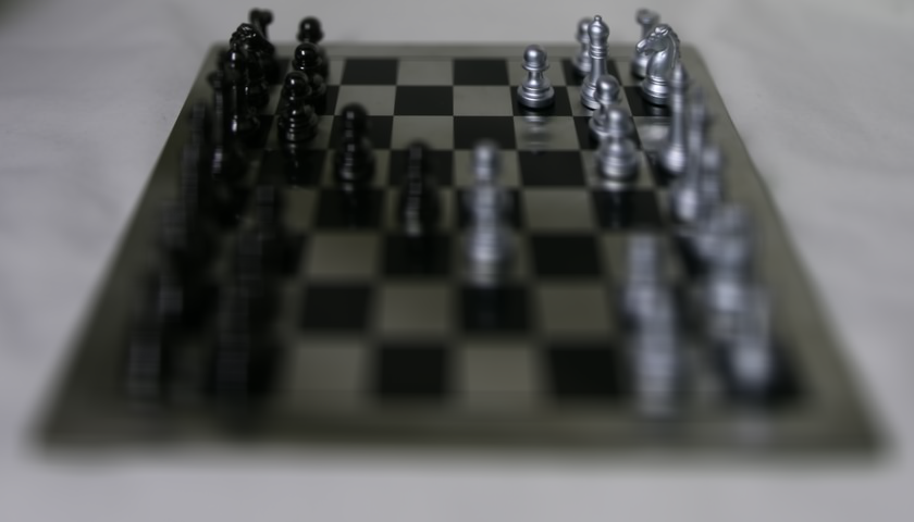
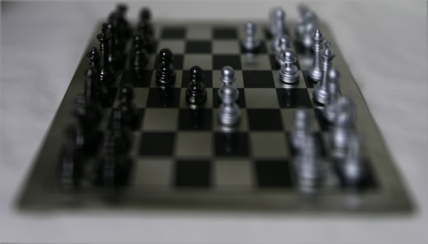
For this project, I reproduced some of the effects explained in the Light Field Photography with a Hand-held Plenoptic Camera paper by Professor Ng using real lightfield data. Through just simple operations of averaging and shifting, we can simulate depth refocusing and aperture adjustment on the images from Stanford Light Field Archive as shown below.Depth Refocusing
When we average all the images in the camera grid, we get an image that is sharp in the back but blurry at the fore-front. For depth refocusing, we can change the focus perspective by shifting the images with a constantalpha and shift image with respect to the image in the center spot of the grid and average the images all together again. Because the image grid from the Stanford Light Field Archive that we are dealing with is a 17 X 17 grid, the center indices will be at (8, 8). For an image at the i, j position, then the vertical and horizontal shift will be alpha * i - 8 and alpha * j - 8. As you can see with the examples below, smaller alpha's focus more towards the back, while larger alpha's focus more towards the front. If the alpha's become too large or too small, then the resulting shifted averaged image becomes a blurry image.
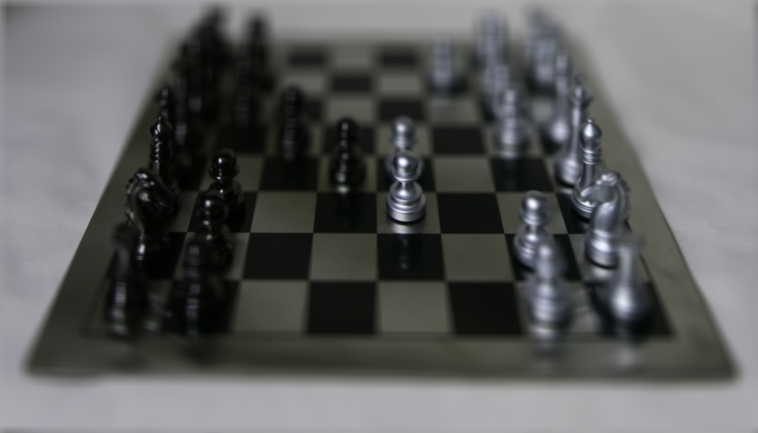

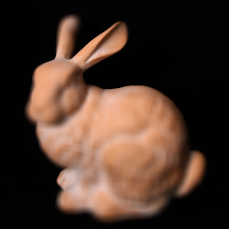
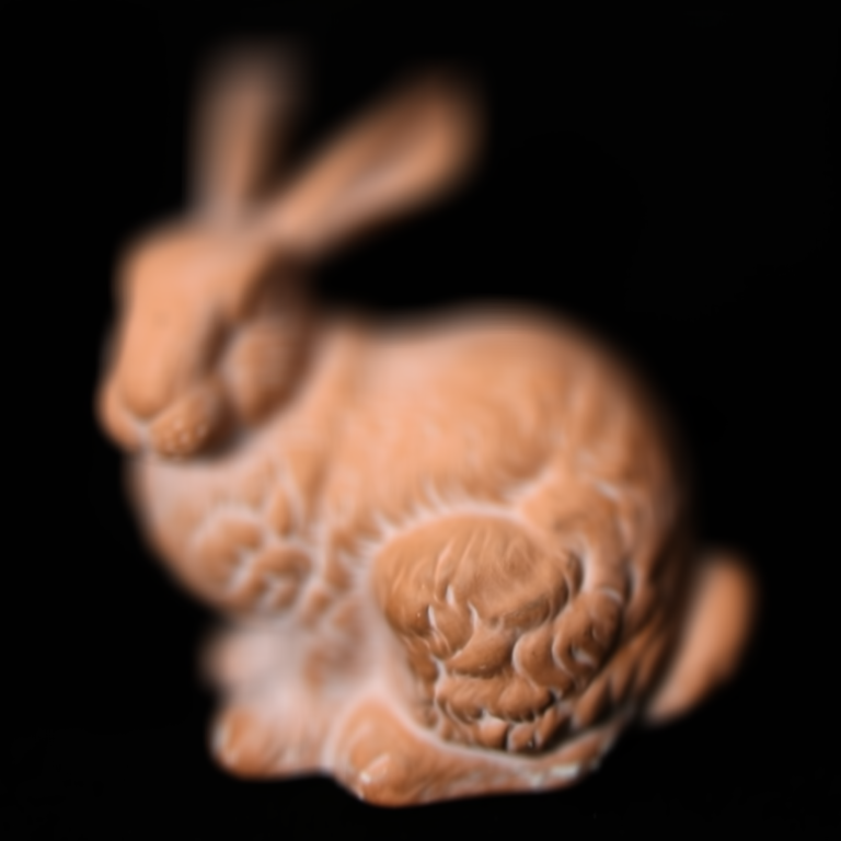
Aperture Adjustment
For aperture adjustment, I added a radiusr constraint to the depth refocusing function, where we will only average the shifted images, which indices' distance to the center is less than or equal to the radius r, in other words sqrt((i-8)**2 + (j-8)**2) <= r. By using a smaller aperture or radius, the image looks focused, but as we increase the aperture or radius, the image starts to focus the depth that we specified.
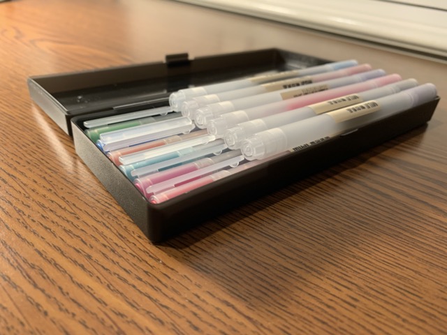
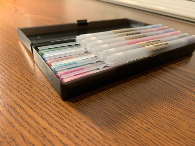
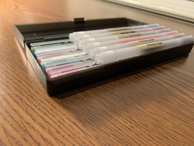
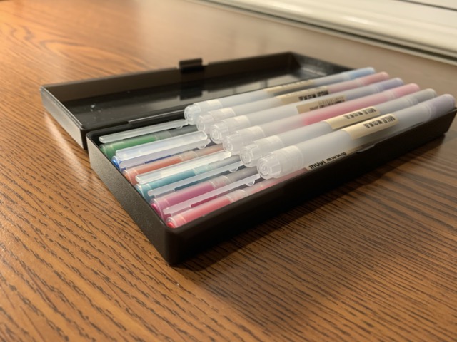
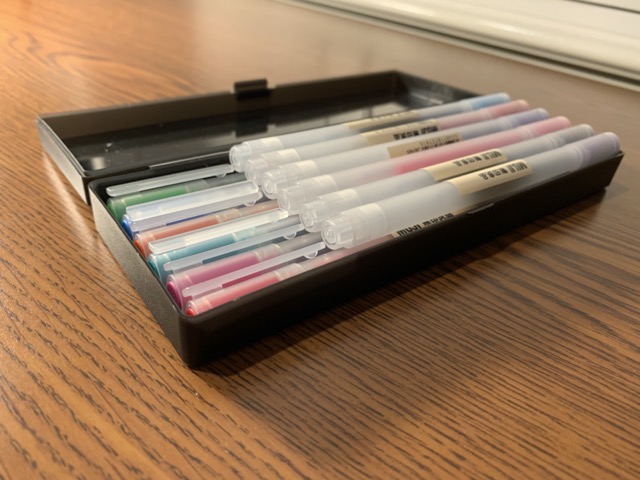
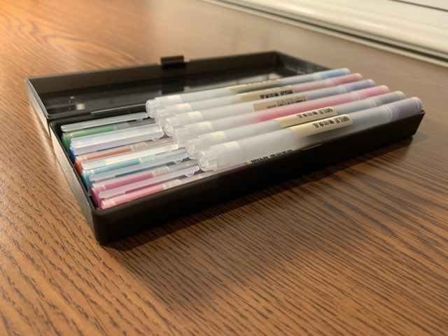
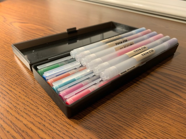
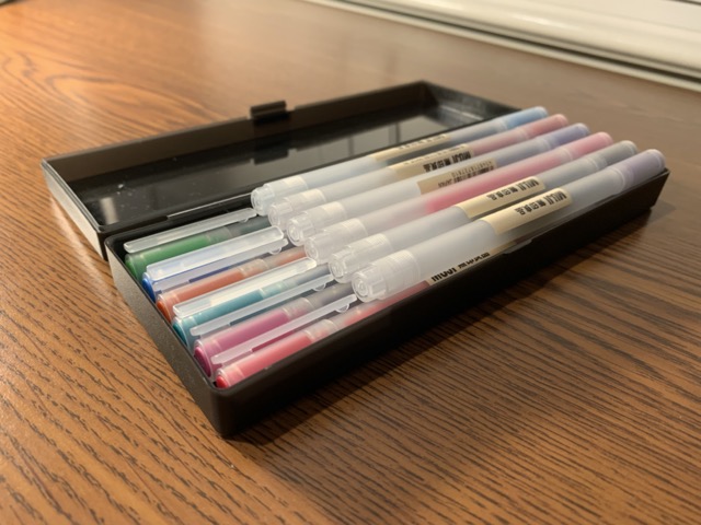
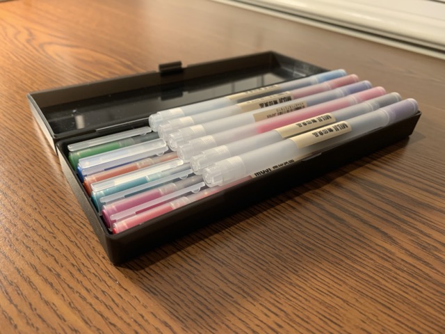
Bells and Whistles
For bells and whistles, I tried taking photos of my Muji Pen box and implemented depth refocusing and aperture adjustment; however, the results look very bad and blurry because I only used 9 images. The depth refocusing barely focused on the Muji Pen labels. Also, I was trying to imitate the lightfield camera data by carefully shifting my hand as I took these photos. I think to improve these results, it would be better if I took a lot more images, like create 6x6 or 7x7 grid instead.