
The goal of this project was to implement an image quilting algorithm for texture synthesis and transfer, described in
this SIGGRAPH 2001 paper
by Efros and Freeman. Texture synthesis is the creation of a larger texture image from a small sample texture.
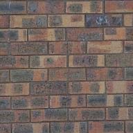
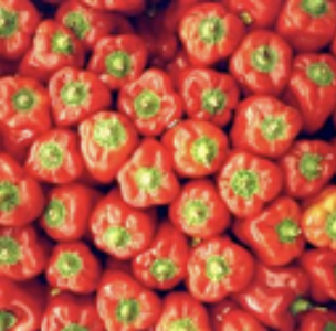
Texture transfer is giving an object the appearance of having the same texture as a sample texture while preserving its basic shape. Below
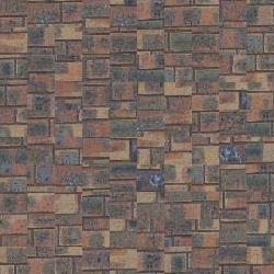
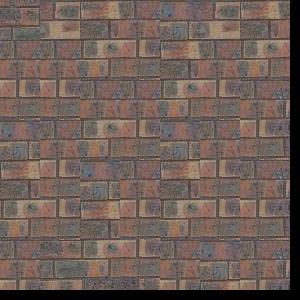
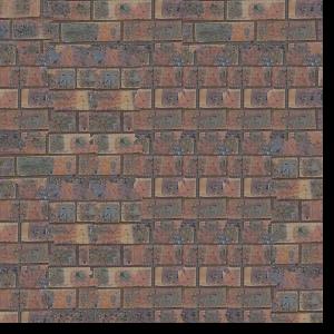
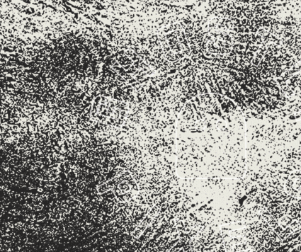
are some sample textures that I used for this project.
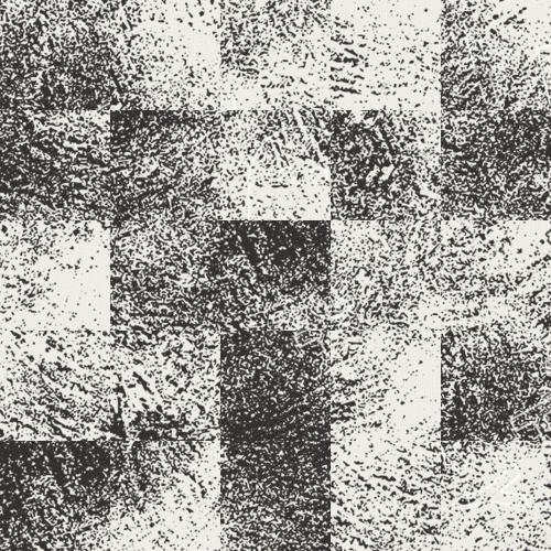
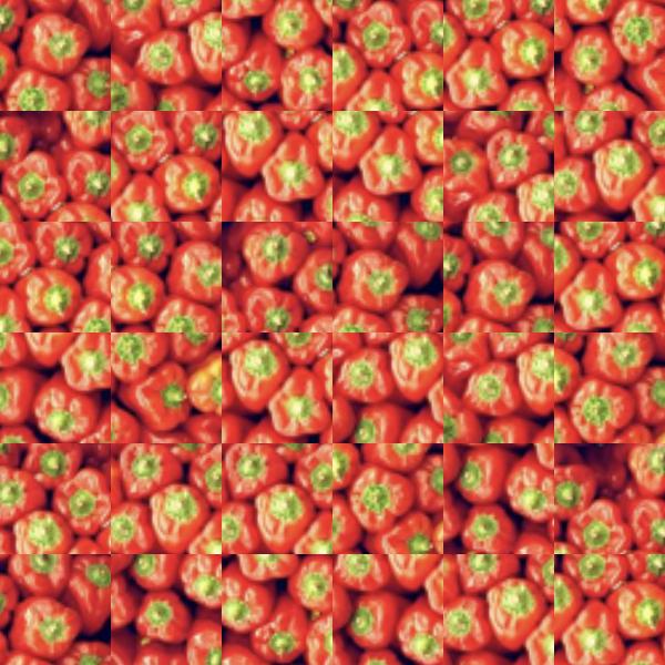
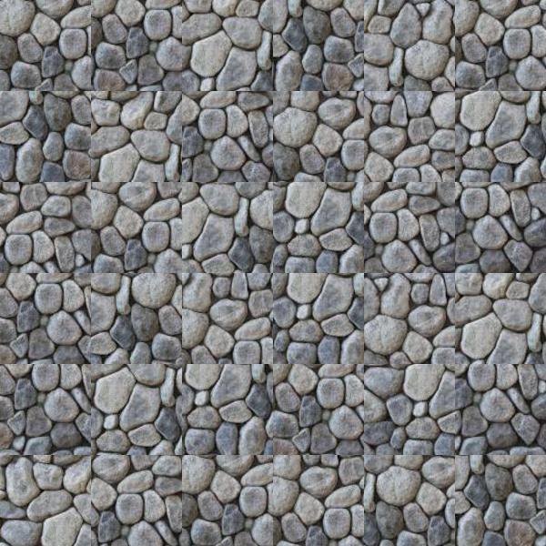
This is the most simple, basic way of texture synthesis. We randomly sample a n x n patch from
the sample texture, and tile the samples until the output image is full. This is simple, but not that effective. Below
are the results of the random patch sampling.
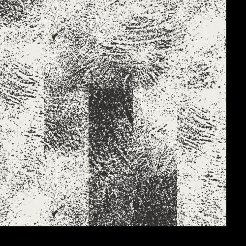
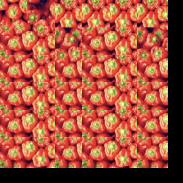
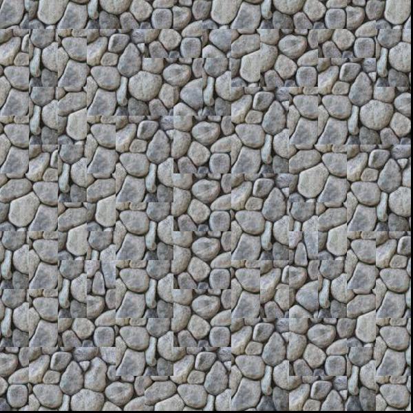
For this method, we first place a random sample in the top left corner. From there, we start finding samples, overlapping
them with the previous sample, and calculate the SSD (sum of squared differences) between the overlapping parts of
each sample patch. We took all the patches within a certain tolerance of the minimum SSD (I picked 1.1, which was recommended),
and chose a random patch from this list of patches. The results were significantly improved.
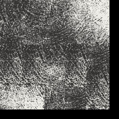
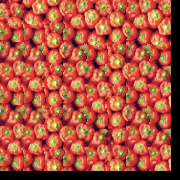
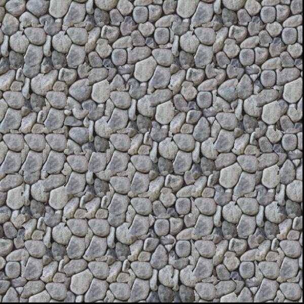
The method finds patches in the same way as method 2, but instead of just placing them right next to each other, we first find
a minimum path in the overlapping region so that the ssd is the smallest, and stitch the image along this minimum path. I used
dynamic programming to find the minimum path, and then stitched them together. The results are similar to the method above, but with
less edge artifacts.
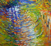
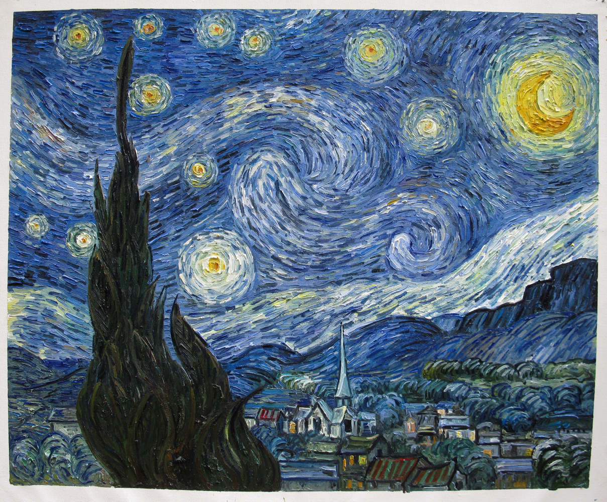
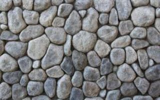
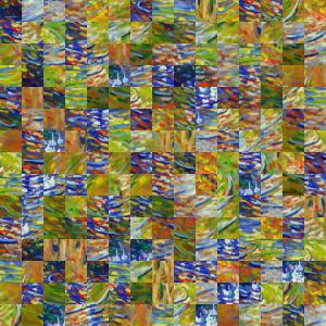
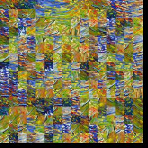
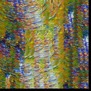
Below are my results on 5 different images. I decided to also run the algorithm on a stone pattern and a grit pattern I found online, and part of
a Claude Monet painting.
From left to right: Sample Texture, Random Patch Texture Synthesis, Overlapping Patches Texture
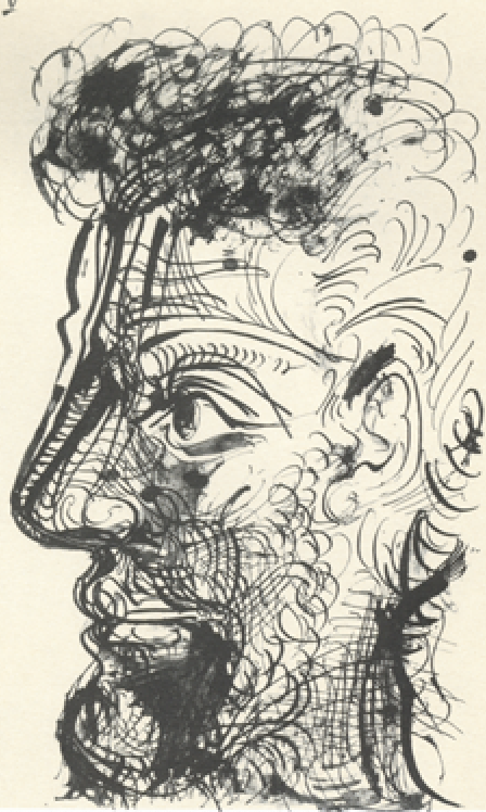
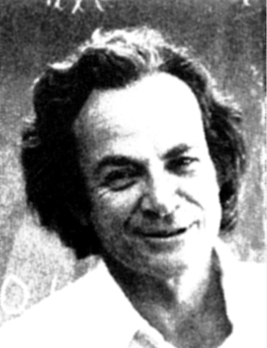
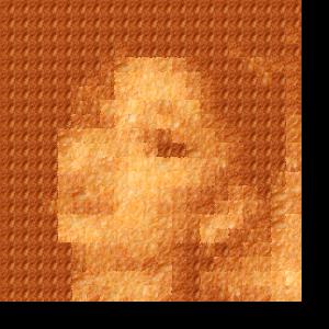
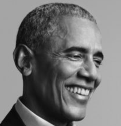
Next, I created an algorithm to transfer a texture onto an image. We can do this by adding one additional cost term to the SSD error function defined in
method 2 based on the difference between the sampled source patch and the target patch at the location to be filled. I later ended up
improving this function with iterative texture transfer.
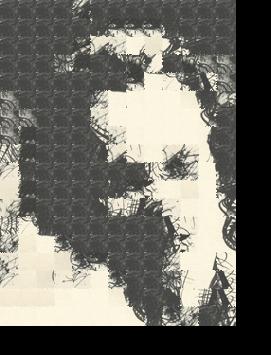
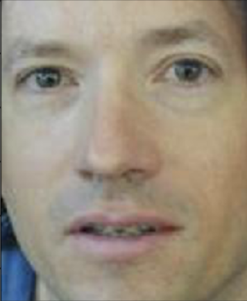
I'm using a relatively large patch size here. With a smaller patch size, we can get a better result - but I decided to just do iterative texture transfer, so stay tuned to how we make our texture transfer even more realistic!
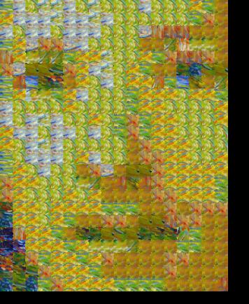
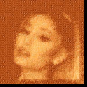
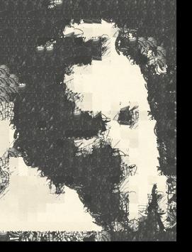
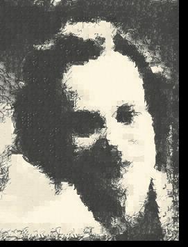
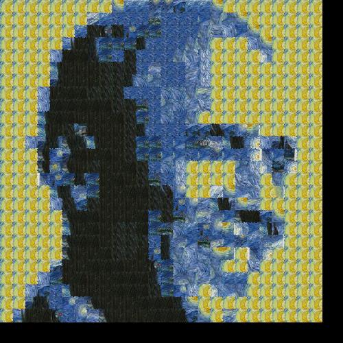
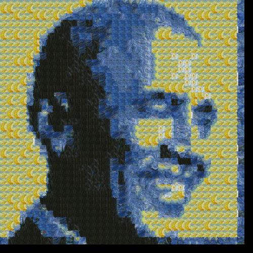
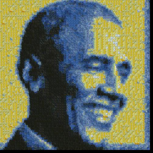
To improve our texture transfer function, I implemented an iterative texture transfer. The only change
from the non-iterative version is that the patches are matched not just with their neighbor
patches on the overlap regions, but also with whatever was synthesized at this patch in the previous iteration, as described in the paper.
This function works by first using larger patches to map out where everything will go, and then using smaller patches to make sure
the textures fit well together. Initially, I used 3 iterations, reduced the patch size by a third each time, and assigned alpha to be
alpha = 0.8*(i-1)/(N-1)+ 0.1, where i is the current iteration and N is the total num_iterations.
However, this took a really long time to run because of my patch size, so I ended up changing my patch size to just decrease by 1/4 each
time.
Results are visualized below.

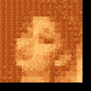
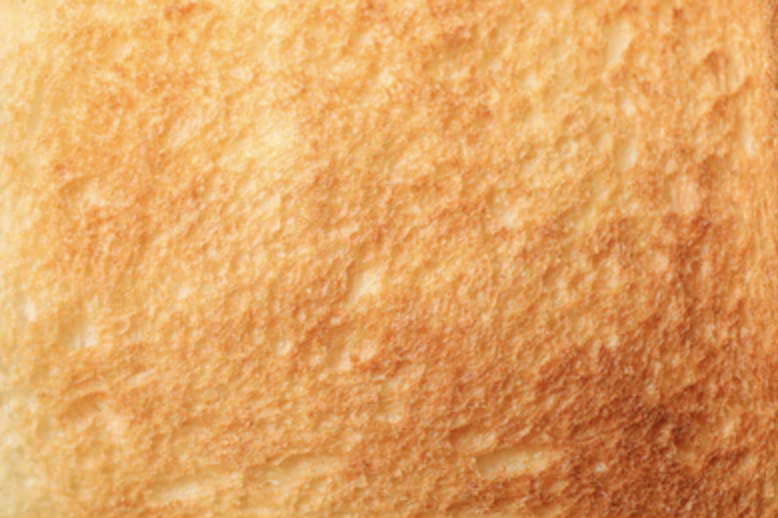
This concepts in this project were really simple to grasp, but a little challenging for me to code because of bugs and alignment issues. I made it out alive and left with some really cool results! I really enjoyed seeing celebrity toast and adaptations of post-impressionist art in the texture transfer part of this projects.
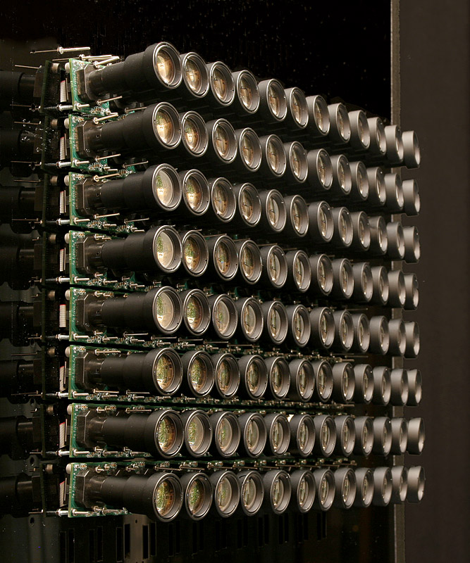
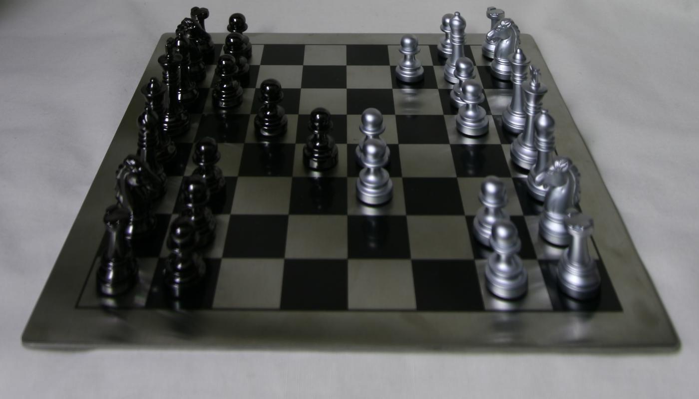
It doesn't stop here folks, we're moving on to the lightfield camera. In this project, I simulated depth refocusing and aperture adjustment with images from the Stanford light field archive, which are images of the same scene taken by cameras that are slightly offsetted from each other. Below is an image of what this would look like (an array of 128 synchronized CMOS video cameras) to help visualize how this is working!
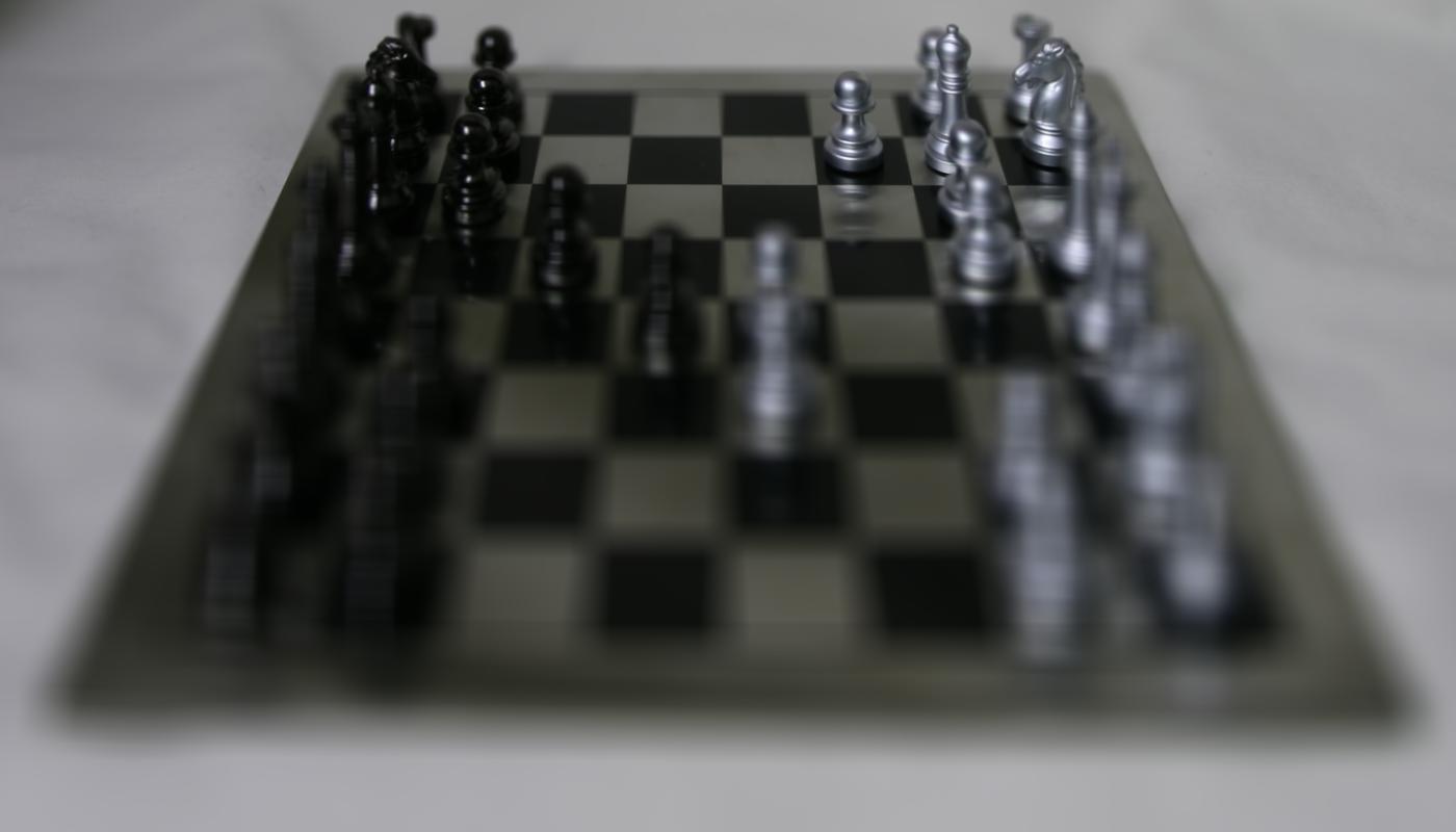
I picked the set of chessboard images from the Stanford light field archive. First, I averaged all the images in the grid without shifting. Since the objects are that far away from the camera don't vary that much in placement when we shift the camera slightly, our resulting image is focused on the far away objects, but has a more blurry view of the objects that are close to the cameras.
Next, I used regex to extract the positions of the cameras from the image names. The average of all the camera positions is
the center of the lightfield camera array, and this ended up matching with the camera at index (8, 8). We used the center camera
coordinates (xc, yc) to calculate the distance between the center camera coordinates and the other camera
coordinates (xi, yi), and end up with
(xc-xi, yc-yi). Then, we pick a shift alpha a and calculate the shift to be a*(xc-xi, yc-yi).
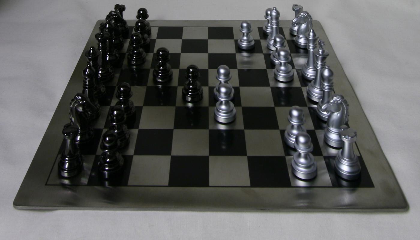
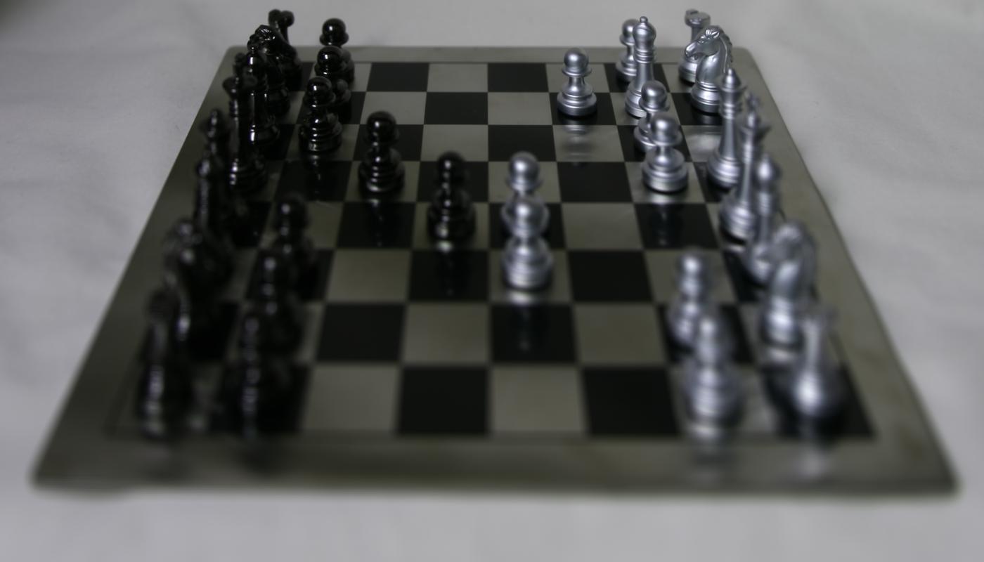
This shifts all the cameras towards or away from the center camera, and refocuses. A larger alpha will give us a clearer
focus on the close objects in the image, and a smaller alpha focuses on the objects that are more far away. I ended up
using alpha values between 0 and 1, as larger and smaller alphas shifted the cameras a bit too far. Below the are results.
Aperture, in a camera, is how wide the hole in the camera expands to let in light. A higher aperture means a larger hole,
and a lower aperture means a smaller hole that lets in a ton of light. Lower aperture is
better when you want everything to be in focus, and a higher aperture lets in lots of light and
gives us a blurry, shallow depth of field effect.
To imitate this concept, I defined a radius r is essentially how "large" the hole in our camera will open.
The larger r is, the more images we want to average. A radius of 5 will take in all the images from cameras
that are located less than 5 points from the center camera. There are a few ways to do this, resulting in different
radii, but I utilized the Euclidean distance for this calculation. A smaller radius will take in fewer images, mimicing a
smaller aperture (small hole). Since there is less displacement among the images, it creates a more focused, sharpened
image. A larger radius (higher aperture, large hole) takes in more images.
Selected results along with a gif are visualized below.

Overall, light fields are really fun to play with and it gave me a new understanding of depth and aperture. I'm surprised by the simiplicity and beauty of this! With just a few simple operations (shifting and average), we're able to modify the aperture and focus of an image with the right data. Am overall really happy with the results, and the learnings along the way.
This class was so fun! It's bittersweet that these were my last projects. I really enjoyed making all of them throughout the semester.