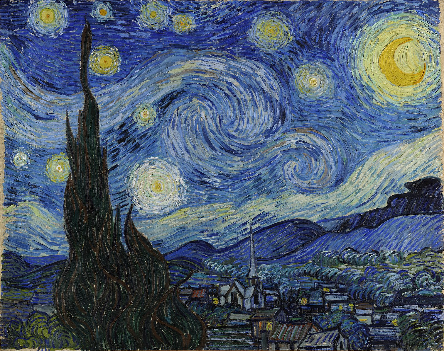
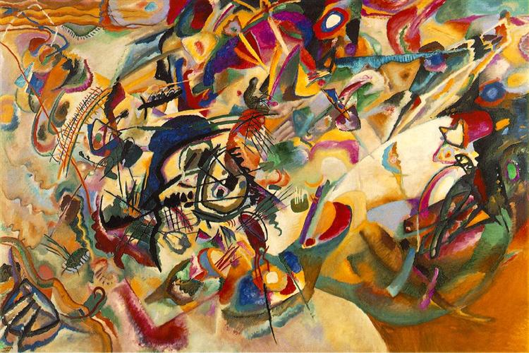
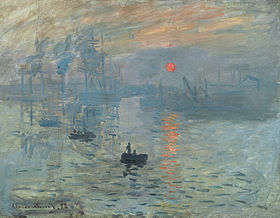
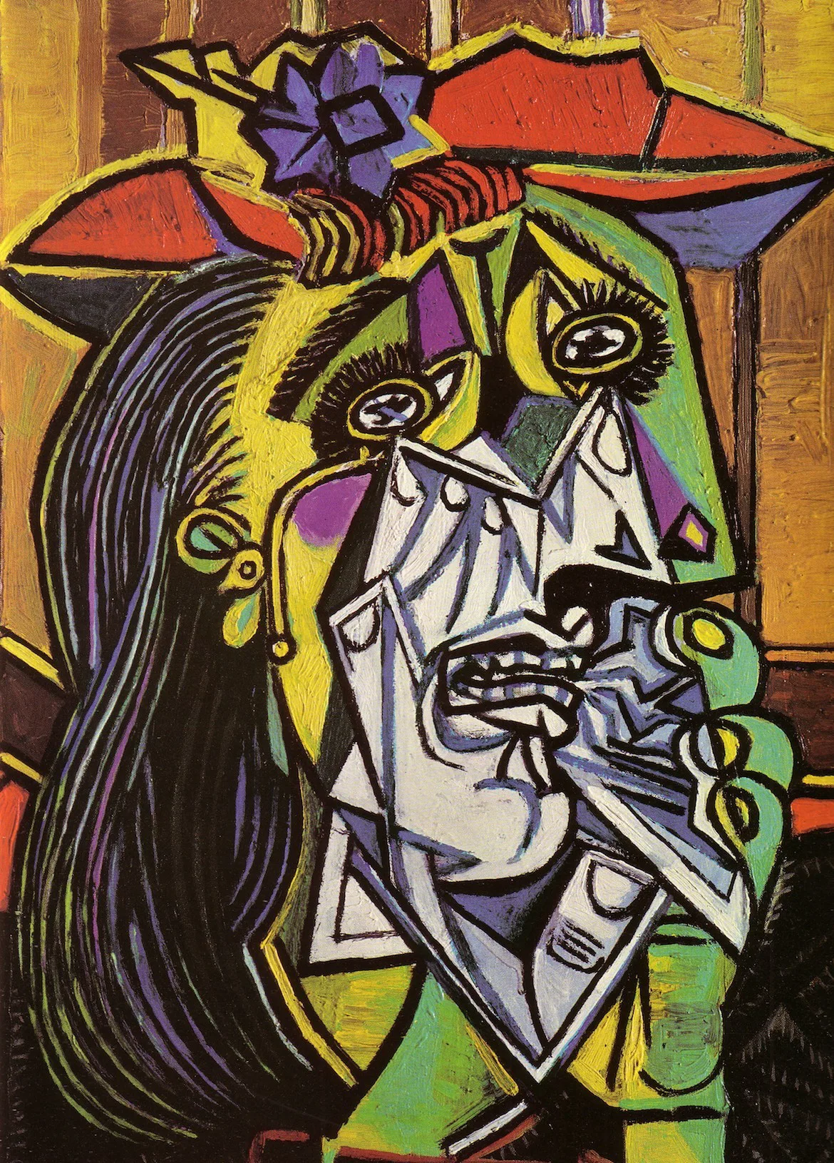
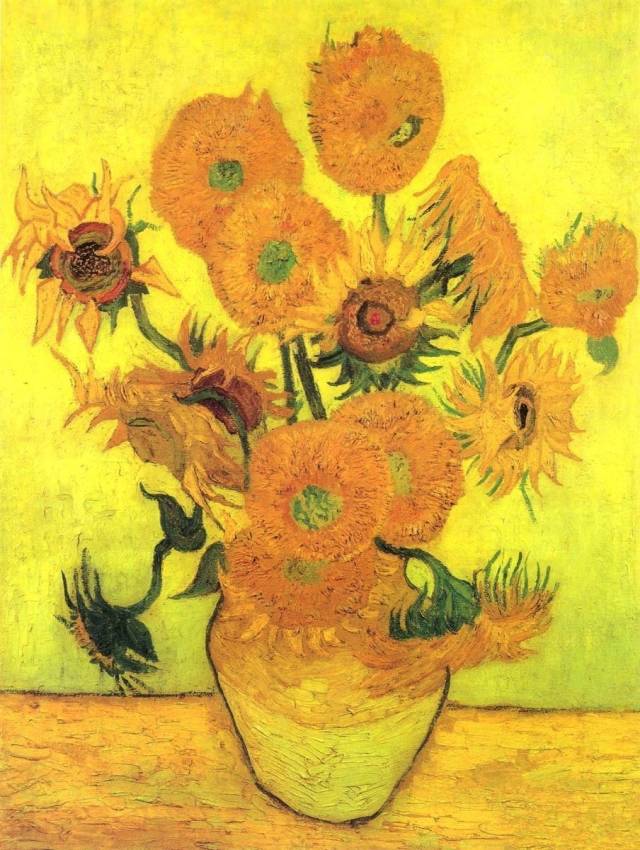
Style Reference
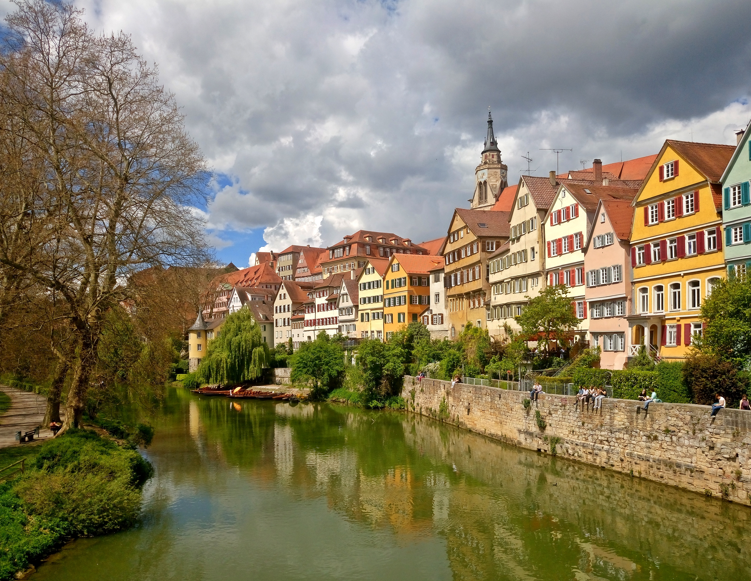
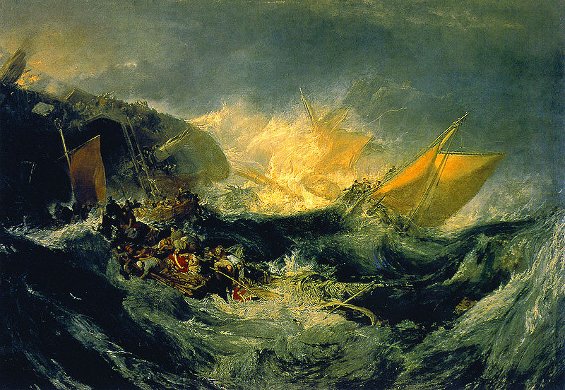
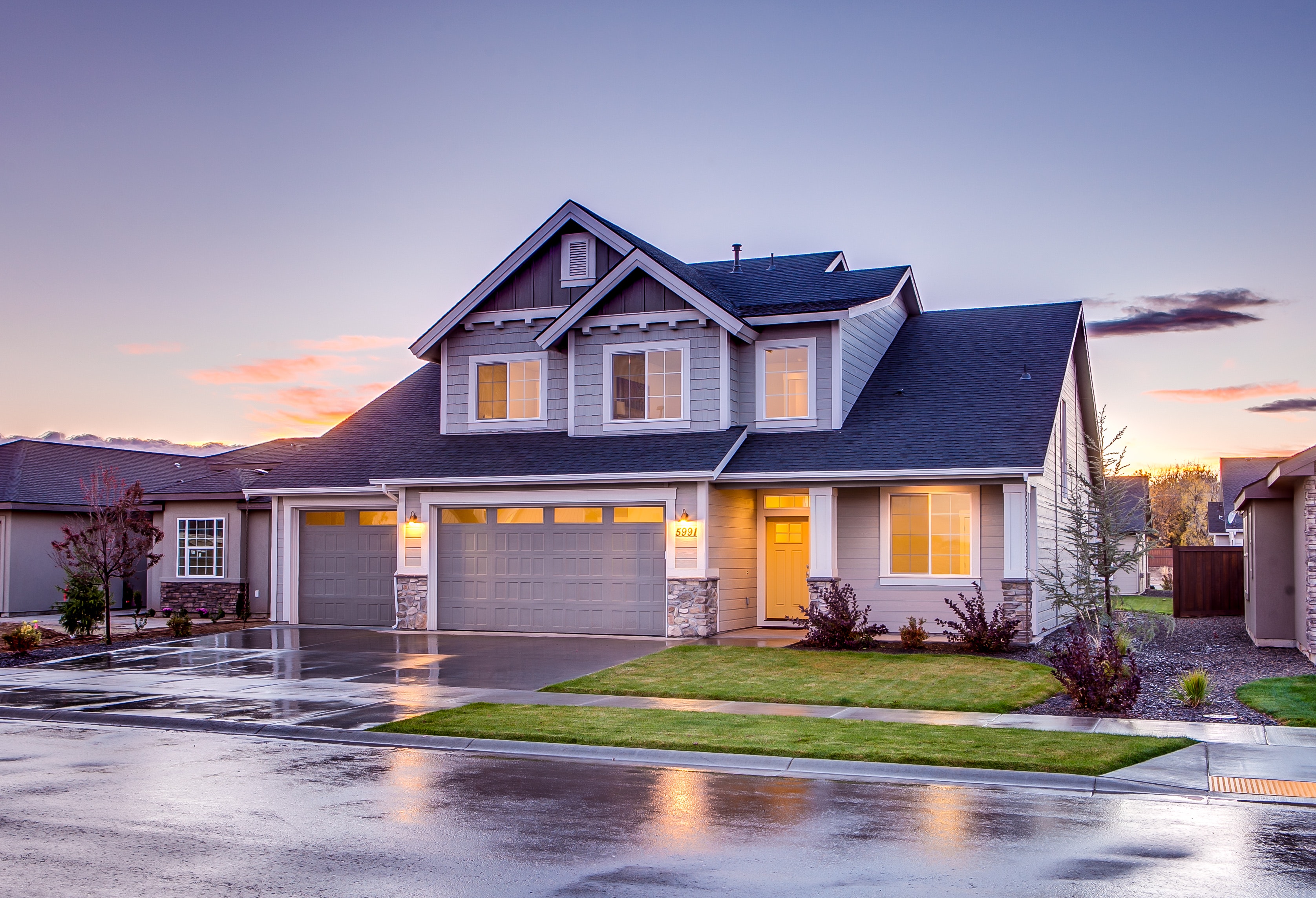
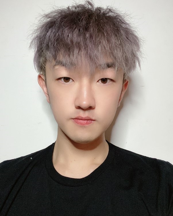
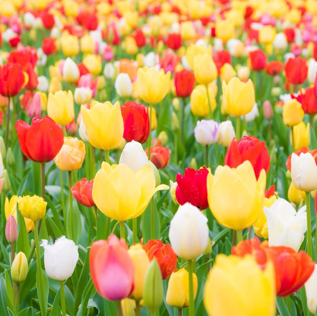
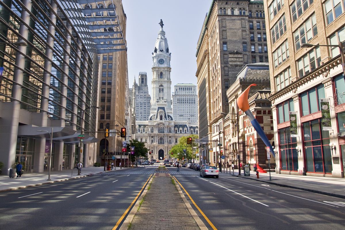
Content Reference
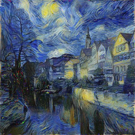
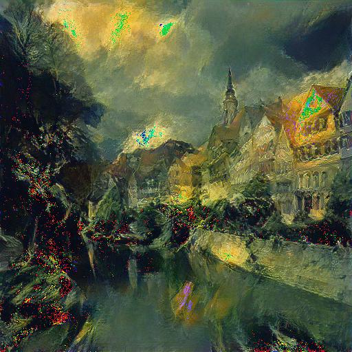
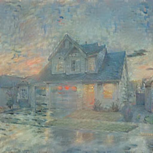
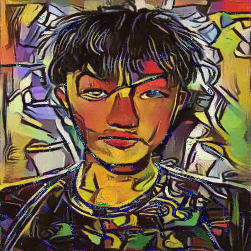
Generated Image
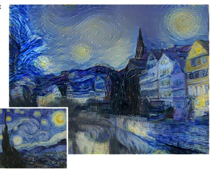
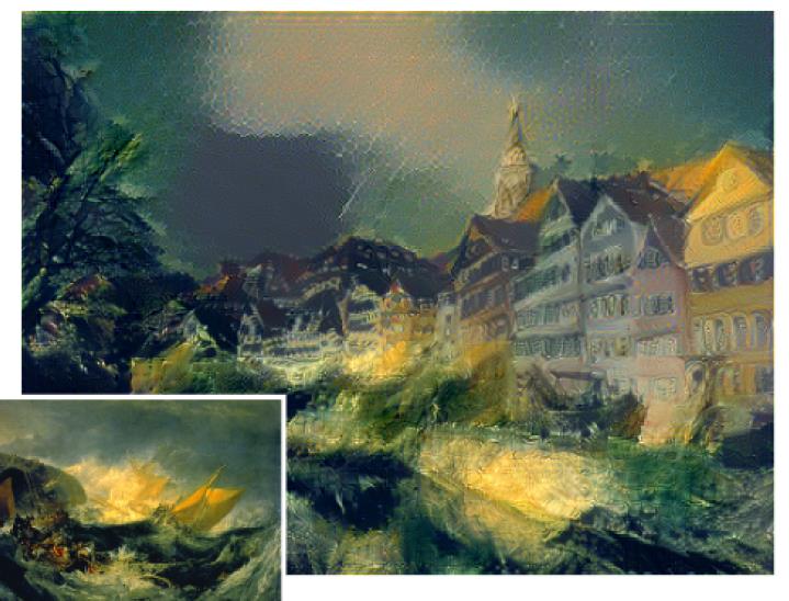
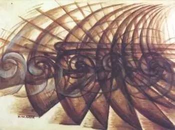
Image in original paper
This project will reimplement the algorithm described in paper A Neural Algorithm of Artistic Style which is used for transforming an artistic style onto any picture and implement neural network learning of the weights.
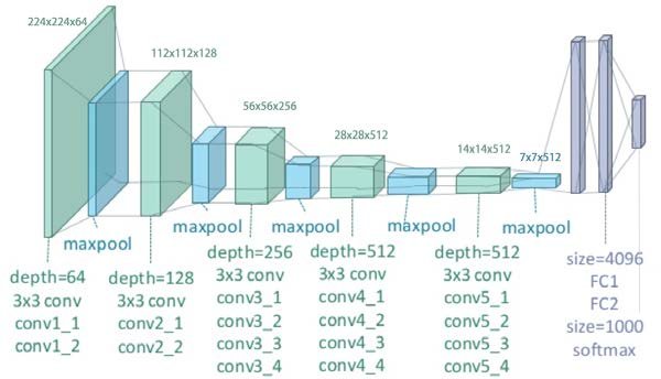
As described in the paper, the project choose to use an open-source neural network, 19-layer non-batchnorm VGG network pretrained on ImageNet dataset (as shown above). However, instead of directing using the whole network as it is, there are several important improvements and modifications mentioned in the paper:
Moreover, the paper provided 5 choices of different subset of CNN layers (a-e) to generate the model for style reconstruction. Here in my reimplementation, I chose plan (e): use `conv1_1`, `conv2_1`, `conv3_1`, `conv4_1`, and `conv5_1` as my subset of CNN for style reconstruction, and use `conv5_1` accordingly for content reconstruction. Therefore, my final neural network has 16 CNN layers, all followed by a ReLU layer and an average pooling layer expect for the last one. There is no full connect layer after the last CNN layer.
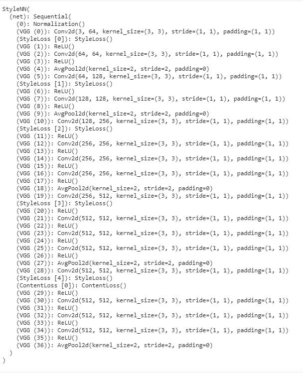
On top of this design, I added couple of layers for better performance and Loss calculation:
My final network structure is as follows:
Given the task, we would like to do change an image to an artistic style while keeping the original content. Therefore, we design two kinds of loss:
Also, in my reimplement, I defined three terms as follows:
While a complete math-wise formula and derivation can be found in paper A Neural Algorithm of Artistic Style Page 9 to Page 12, here I would like to conceptualized the method of getting losses described in the paper and talk about how I implemented them in my project
For content loss, we only look at the loss generated at the first CNN layer of the last block `conv5_1` as proposed by the paper. The loss is defined as pixel-wise MSE loss of between the input image after going through all layers of our network and the content reference image after going through all layers of our network. In order to calculate this loss, I added a content loss layer after the final CNN layer in the network as a Loss layer.
For style loss, it is defined as the sum of all losses at the first CNN layer of each block. Each layer's loss is defined as the MSE between the respective style representation matrix of the input image and the style reference image at that layer. The style representation matrix at layer l is defined as the inner product between the vectorised feature map of image outputted at layer l. In order to calculate this, I added a style loss layer after each CNN layer and calculate the respective loss at each CNN layers.
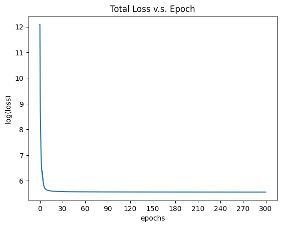
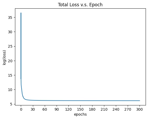
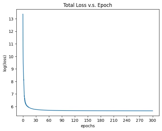
The total loss is defined as the weighted sum of Style Loss and Content Loss. Different ratio of the weight of style loss over the weight of content loss will give different output result. A higher ratio will lean towards getting more similar style, while lower ratio will lean towards getting more similar content. By looking at the figure 3 in the original paper and run several experiments, I chose to use ratio 10^(-6) to get the best result. Also, for better visualization of loss plot, I chose to use 10^9 and 10^3 as my final weight for style loss and content loss respectively. Thereafter, I used LBFGS optimizer as my network's optimizer and change the input image accordingly with respect to the total loss. I defined the process of backward tracing and training of network as my closure function and by the nature of LBFGS optimizer, I chose to train the network for 30 epochs to get my final result.
First, I transferred Neckarfront to the following three styles mentioned in paper, and made comparisons with the ones in paper:
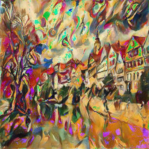
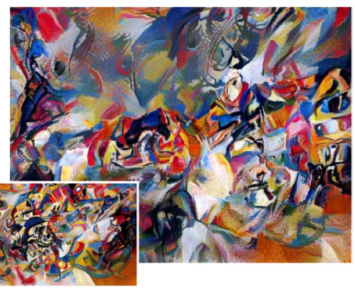
The followings are several examples of my generated images through the network I defined.
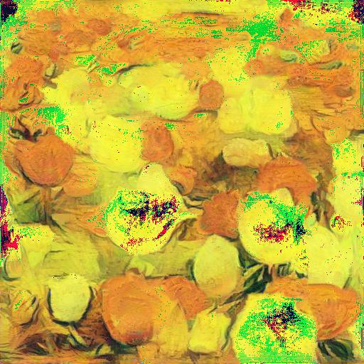

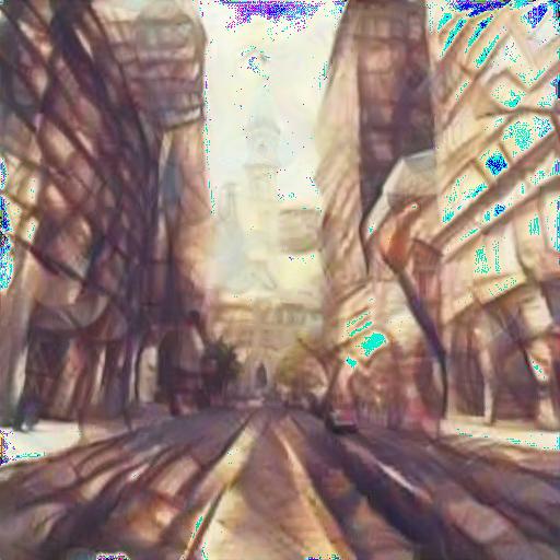
For all the results I get above, most of them works extremely well expect for some of them have weird color spots. For example when we want to transfer the city image to Bala's style in the last example. One possible reason for this is that the style reference image is too monotonic while the content image contains too many color components. As a result, the network will get confused and output weird color spots.
Most of the results above are very pleasing except for the Femme_nue artistic style. There can be several reasons for this defect. One most possible reason is that the use of color in the original style picture is too monotonic, which resulted in the mean/sd of the image not following the mean/sd provided by ImageNet. Therefore, the normalization process changed some pixels of the original image and led to the defects.
Overall, the project is very interesting and motivated me to explored a completely new field that can be achieved through computer vision and deep learning. When studying and preparing for this project, I also noticed that there are many improvements to the paper we reimplemented here later and I would like to further explore them to get more updated on this field.
This part, will we follow the idea demonstrated in this paper by Ng et al. to reproduce some of the effects using real lightfield data.
In this project, I used the data from Stanford Light Field Archive as the lightfield image data. Specifically, I chose three of them to do the following parts:
For depth refocusing, I took all images provided by the dataset archive and used them all to "average out" images focusing on different depth. Importantly, since the dataset provided changes in different rotation direction, I take this factor into account when building my project for depth refocusing. Also, through multiple experiments on different dataset, I also find out that the scaling factor we should use for refocusing highly depends on the complexity of the image's content. When there are many contents at many different levels (such as in the gem box dataset), the scaling factors can spread more widely. On the other hand, when the content is simple as in the purple gem dataset, the scaling factors should be more closed around 0.
After setting the scaling factor, the refocusing algorithm aims to find the horizontal and vertical offset of the current image to the center image. Since the image indices are provided as part of the file name, I figured out the offset in x and y direction and then shift images to align with the center image by manipulating the numpy image matrices with respect to x/y offset, scaling factor, and image direction. Thereafter, I averaged across all aligned images to get a final result at one scaling factor. After generating all images, I output them all in order to a gif file shown below.
For aperture adjustment, the target is to set a radius r and find is a current picture is inside this aperture radius. After checking if the offset in x and y direction is in a circle center at the center of the grid, I averaged across all images laying in side the circle to get the image at this aperture radius. After generating all images, I output them all in order to a gif file shown below. The values of the radii are also chosen through running multiple experiments on each dataset.
The final results are shown as below:
Through this project, I found out that how interesting it is to implement a seemingly complex and complicated idea with rather straightforward and simple algorithm. Also, the application of this project is broad and I believe further studies on subjects such as manipulating light field data could be very impressive.
As part of the bells & whistles, I implemented interactive refocusing. First, the user can choose an arbitrary at the center indexed image. Thereafter, each of the other images are shifted with respect to the point's coordinate. The image's coordinates are also provided as part of their file name. Since the images are provided in a regular grid structure, I only need to find a shift of one image and then align all other images with respect to that image under the corresponding grid-offset. The final result is shown as follows:
For this part, I shot several images with the camera of my cell phone and ran refocusing / aperture adjustment on the images I shot. The result is shown as follows:
The result is not very pleasing as many frames are very blurry. I think there are mainly two reasons. First of all, I only took about 100 images in the same way as Stanford's archive, which is about only have the amount. Therefore, the averaging process may not be very representative as the whole image. Second, I tried my best to hold the camera still when moving it, but there still could be offsets in when I took the images. Third, I used my cell phone's camera instead of a profession one that can be more precise focuses and so on. As a result, there are too many noises in my data, so the result is the case above.