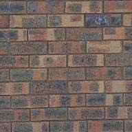
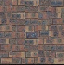
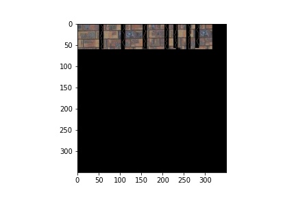
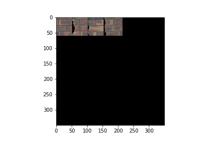
First, I randomly selected a patch from the image. This leaves to large artifacts. Next, I implemented
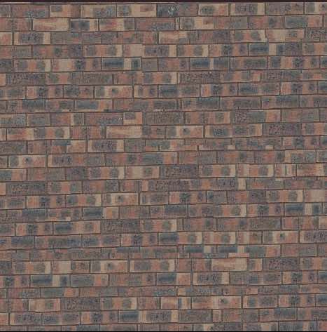
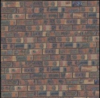
overlapping patches which selected an optimal patch based on the SSD in the overlapping region. Any patches
within some tolerance of the mininmum possible error could be randomly selected. Finally, I implemented seam
finding which I will explain in the next section.
Original BricksRandom BricksBricks w/ OverlappingBricks w/ Seam Finding
Seam Finding
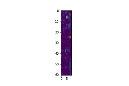
First, we compute the SSD between 2 patches at the overlapping region. Below is an example for the vertical seam
case.
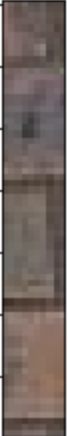
Overlapping Brick Patch on the left (already in image)Overlapping Brick Patch on the right (incoming patch)Seam SSD
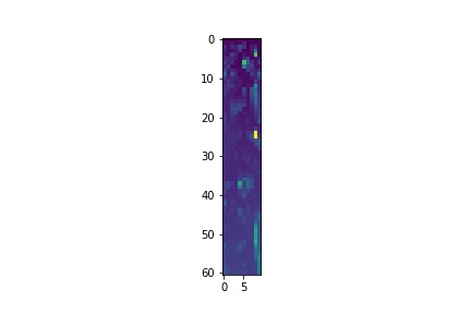
Next, we compute the cost of various paths using dynamic programming. Below is a visualization. We can backtrack
through this array to find an optimal vertical cut that has the least cost.
Seam DP
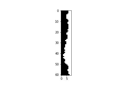
Once we have a cheapest path, we create a mask by assigning all points to the left of the path as 0 and to the
right of the path as 1.
Mask
Below is a visualization of the output where we set a mask where the path is 1 and everything else is 0.
Boundaries in the Output
Below is a different visualization where we only include the portions in overlapping regions that come from the
right-side patch.
Boundaries in the Output
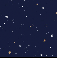
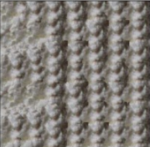
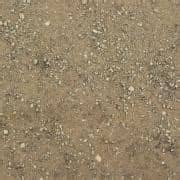
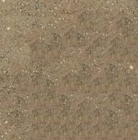
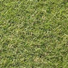
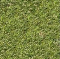
Some more examples of image quilting
Original SkyQuilted SkyOriginal White SmallQuilted White SmallOriginal DirtQuilted DirtOriginal GrassQuilted Grass
Texture Transfer
In this part, I transfer the texture of one image to another image using a similar strategy to image quiling. In
order to accomplish this, we modify the error function to include the error between a texture patch and the
corresponding image in the original image.
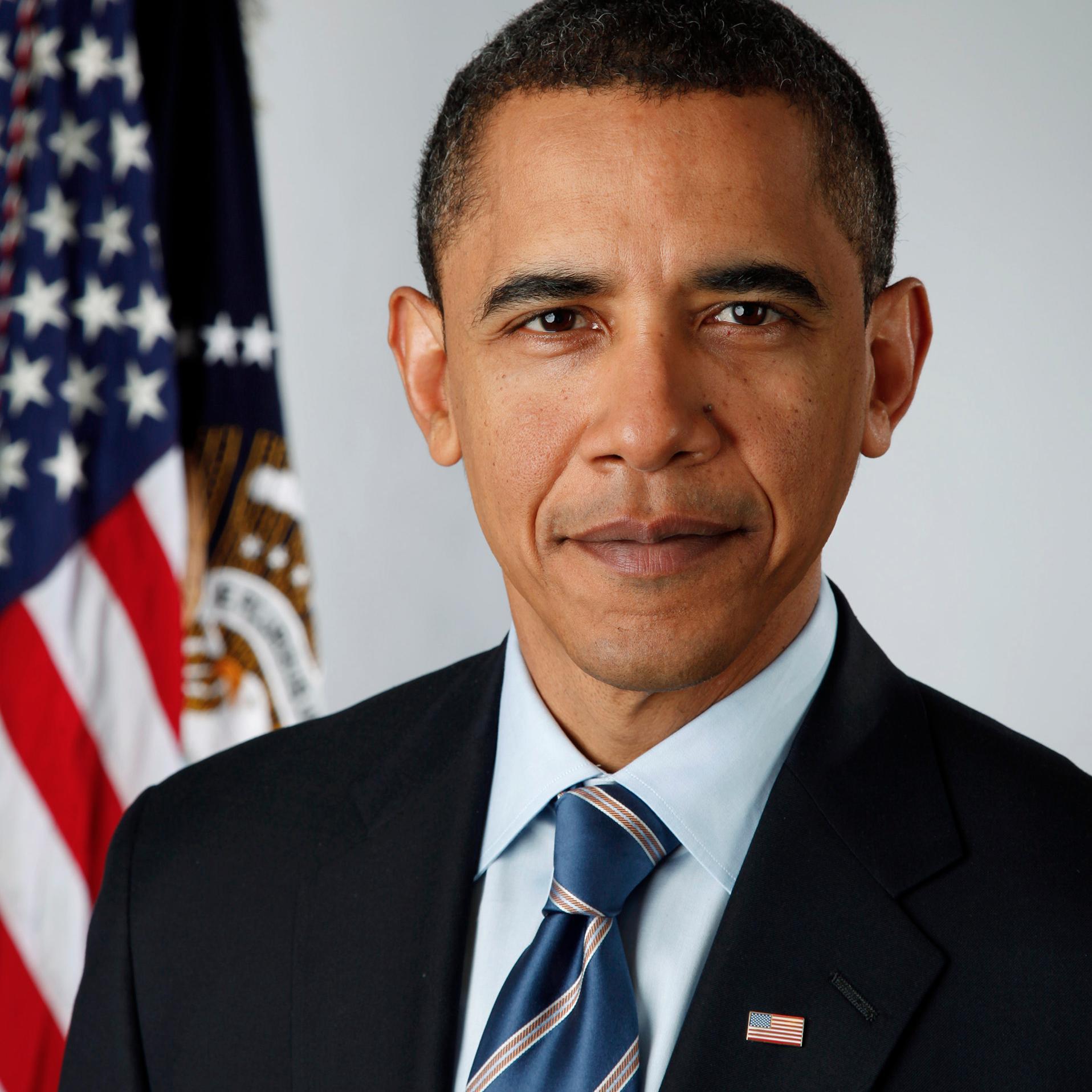
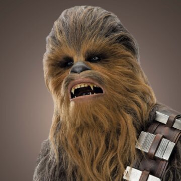
White TextureObama ImageTexture Transfer ObamaChewbacca ImageTexture Transfer Chewbacca
Bells and Whistles: Implementing cut.m
I implemented my own version of cut.m by writing 2 functions to handle vertical and horizontal seams separately.
I would apply the vertical seam first (if it was not the first column of the output image) and then would apply
the horizontal seam (if it was not the first row of the output image). The output of my cut functions (which are
named vertical/horizontal seam) is a mask that I use to determine whether to use the left or right side of the
overlap.
Overall, one of the tricky pieces of this project and a great learning was how the various ways we could get
some small runtime speedups like computing SSD in parts and caching parts instead of recomputing for every loop.
Additionally, I learned some of the tradeoffs between quality and speed due to playing around with the patchsize
and overlap. Thanks for a super fun project.
Lightfield Camera
Depth Refocusing
The goal of this section is to be able to shift images from the Standford Light Field Archive dataset in order
to replicate the effects of changing the depth of focus of a camera. We accomplish the case of focusing on far
away parts of the image by doing a simple average of all of the images in the dataset. For the case where we
want to focus at different levels, we shift the image based on its location in the camera grid towards or away
from the center based on a focus scaling factor that we input.
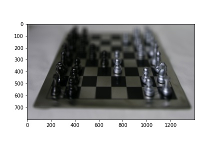
In the below gif, we can see how the "camera" focuses on the front of the image of the chessboard and then
focuses step by step on
a farther region.
Chess Refocusing: -3 to 1
We can see a similar result on the jellybeans.
Jelly Refocusing: -3 to 6
Aperture Adjustment
In this part, we want to replicate the effects of different sized apertures around the center of the image.
We implement this by creating a circular mask with a size of the aperature radius and only applying the
depth refocusing style averaging (averaging with the shift towards/away from center) to the images that are
in the circle.
We can see the effect of increasing the size of the aperture on the chessboard image.
Chess Aperture: 1 to 8
We can also see its effect on the jellybean image
Jelly Aperture: 1 to 8
Bells and Whistles: Interactive Refocusing
For this section, I took an input from the user about the section they wanted to focus on and applied a shift
based on that input. Below is an example of the refocusing on a point in the bottom-right region.
Interactive Refocusing on the chessboard
Overall, I enjoyed getting a better "physical intuition" of how different focal lengths and apertures affect the
appearance of the image. I also am glad to have learned about the Lytro camera. It is exciting to know that
there are still new simple novelties to be developed in the imaging field.