CS-194-26: Final Project 1 (Lightfield Array)¶

Abhijay Bhatnagar¶

Part 1: Depth Refocusing¶

Given the Stanford Lightfield Array images, we have a rich set of images taken slightly displaced from each other, giving us an ample amount of depth data. We will extract the relative positions of each image embedded in the file name and use that to focus depth at various positions.

Average Image¶

We start by taking the naive average of all of the images without any shifting. This should provide a depth effect with the foreground blurred and the background in focus.

<matplotlib.image.AxesImage at 0x13082ac90>

For our own sake, we will compute the average position of the camera and use that to center the camera's coordinate positions of each image.

The average position of the camera is: [-818.30 -3314.06]

Depth Refocusing¶

For our refocusing procedure, we will use the provided grid structure of the lightfield array to calculate the displacement from the center. By parameterizing this displacement, we can align the images to focus on different sections. Our ideal range from bottom to top is $[3,1]$.

The images of different focuses are provided below.

Aperture Adjustment¶

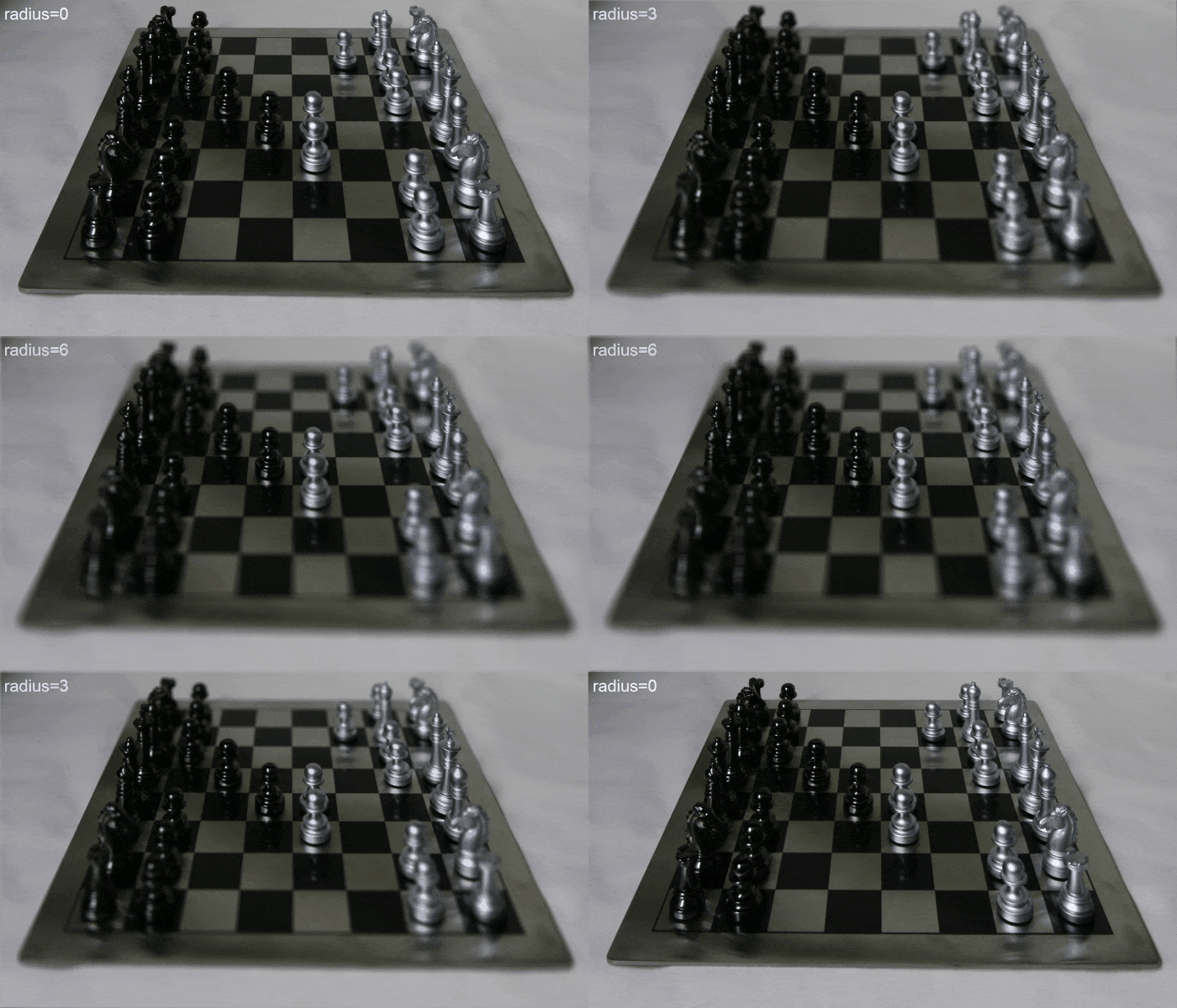
Here we will simulate an artificial aperature by filtering and averaging images in a perpendicular radius of a chose size. As we increase the simulated aperature, we expect the imgur to blur around the edges, as in a real camera that would become unfocused.

For demonstration purposes, we have set the depth of focus to be in the middle of the chessboard.

What did I learn¶

I learned that it is surprisingly straightforward to use an array of images to achieve remarkably cool effects, and through the combination of many similar images, we can actually simulate camera features.

CS-194-26: Final Project 2 (Texture Transfer)¶

Abhijay Bhatnagar¶

Part 1: Randomly Sampled Texture¶

To begin the project, we will create a quilt from samples of existing textures. We are working with the following provided textures.

From these, it is fairly trivial to select random square textures.

And with these random samples, it is pretty straightforward to piece these together to create a randomly sampled quilt.

Part 2: Overlapping Patches¶

Clearly these quilts don't look all that cohesive. To improve this, we can overlap patches our patches by a slight margin, and pick a sample that matches the overlapped region within a tolerance level. We can used ssd to compute a cost minimisation metric to choose candidates for that sample, and we can generate masks relative to a horizontal and/or vertical overlap to properly focus on the relevant regions. As an additional challenge, I attempted to generate complete quilts with no black border, regardless of sample or quilt size. This required a decent amount of work in making the masks and samples agree in dimensions around the borders.

The results on the 5 textures are shown below, with the best one (the bricks) emphasized.

<matplotlib.image.AxesImage at 0x1339327d0>

This process works quite well for textures that have high visual similarity, such as the bricks or the words, where there are many similar overlapping regions. It works much worse for images that are feature-rich, such as the human face, as the overlaps are less helpful.

Part 3: Seam Finding¶

Based on the flaws of the previous method, there is a lot of room to improve, particularly between the borders of different patches. To improve this, we can compute the min-cost cut between two overlapping regions, and merge the patch into the greater quilt along that cut.

Seam Explanation¶

Create an illustration of the seam finding. Include three images: the two overlapping patches and the cost (squared difference). On top of the cost image, plot the min-cost path. The cost image can be displayed with imagesc with axis image and the path plotted using hold on, plot. You can edit cut.m to create this display or to output the path to display:

To begin with, we will showcase how the seam-finding works at one random patch. First let's take a look at the quilt so far.

<matplotlib.image.AxesImage at 0x1305ec550>

Here, the first row has been complete filled, and we are now adding the first patch on the second row. Let's take a look at that location.

Here are the same images but cropped to the overlapping region.

Now the real magic comes from computing the min cut of that cost_image. We will traverse the columns and compute the lowest-cost connection between the columns, and the set of these connections forms the min-cut. This is illustrated below.

Now let's see the corresponding cuts on the overlapping regions.

The natural step is to merge these two cut regions...

Now we can see this visualized on the entire patch

Text(0.5, 1.0, 'Merged, uncropped')

From here, we can now add this to our quilt, and we are done!

Quilt Cuts¶

Now let's see this in action. I've visualized the quilt cuts on our provided textures, and for added fun, I've included a graph of all of the min cut borders presented as masks between the original canvas (black, at the point that region is being modified) and the incoming sample (white). See if you can use that to spot any seams.

Here are the results on a couple textures of my choosing. You can see how you can really expand a pattern using this technique.

Quilting comparison¶

For comparison, here are the three quilting techniques side by side.

Part 4: Texture Transfer¶

Now that we've built the core of technology, we can actually convert this to a texture transfer tool really easily. If we change our cost function to calculate the SSD between the sample and the target image, we can take the samples that best match the target image, allowing us to 'transfer' the texture. If we parameterize this cost to mix both the target and current quilt, we can achieve intermediate texture maps.

<Figure size 1440x720 with 0 Axes>

Bells and Whistles¶

Face in Toast¶

For putting my face in toast, I'm going to combine this project with project 2, and use gaussian / laplacian blending with a transferred texture to achieve facial toasting.

First, here are my baseline images...

Now I ended up experimenting with a bunch of different transformations on my face in order for the transferred texture to have the right color balance for a successful blend. It needed to have a perfect balance of dark features but not overpoweringly dark edges. Here are some of my attempts...

For my blending, I ended up going with the last attempt on the right. Here is my gaussian / laplacian blending code:

def make_gstack(img, ksize=25, sigma=2, levels=5):
    G = cv2.getGaussianKernel(ksize, sigma)
    G = G @ G.T

    stack = [img]
    for i in range(levels):
        blur_c = lambda c : signal.convolve(stack[i][:, :, c], G, mode="same")
        stack.append(np.dstack([blur_c(c) for c in [0, 1, 2]]))
    return stack[1:]
def make_lstack(img, ksize=25, sigma=2, levels=5):
    gstack = make_gstack(img, ksize, sigma, levels)
    stack = [img]
    last = img
    for i in range(0, levels - 1):
        lp = (last - gstack[i])
        last = gstack[i]
        stack.append(lp)
    stack.append(gstack[-1])
    return stack[1:]
def blend(img1, img2, mask):
    L1, L2 = make_lstack(img1), make_lstack(img2)
    G = make_gstack(mask)
    LS = []
    for i in range(len(L1)):
        LS.append(G[i]*L1[i] + (1-G[i])*L2[i])
    return sum(LS)

Clipping input data to the valid range for imshow with RGB data ([0..1] for floats or [0..255] for integers).

Custom Cut Function¶

For my custom cut function, I struggled to make it work effectively. However, I attempted to implement Edmonds-Karp max flow on the cost image represented as a graph. The construction for a horizontal cut is as follows:

For each pixel of a column of the image cost, connect a directed edge between the pixel and every pixel of the next column. Assign each edge a weight equivalent to the cost of the target pixel.
Connect a source node to each pixel in the first column. Assign each edge a weight equivalent to the cost of the target pixel.
Connect a sink node to each pixel in the last column. Assign a weight of zero.
Run a Max-Flow / Min-Cut solver.

This will return the minimum cut. For a vertical cut, simply transpose the inputs.