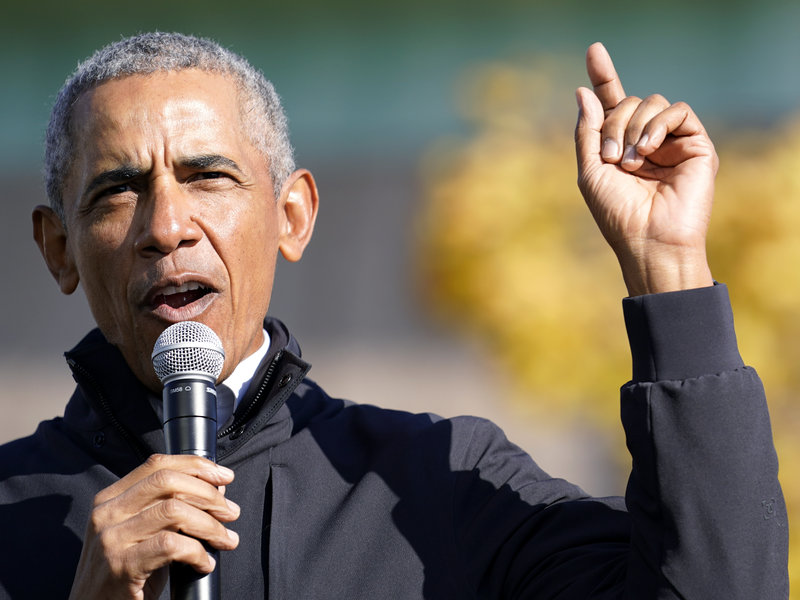
Project 1: Light Field Camera

This project focuses on creating a light field camera by taking a series of images on a grid, shifting them using a scale and a reference to the center image, and averaging them together. In doing so, we can create images that focuses at a certain depth of field while blurring other depths. We can see this using refocusing and aperture adjustment.

Depth Refocusing

To focus in at certain depths, we construct a grid of the images. We do this by sorting the image names in order and arranging them on a grid. In the following set, we use a 17 x 17 grid. After this, we shift the image based on its location in the grid and its distance from the center image, and multiply this by a certain scaling factor, which determines which depth of field to focus on. In the following results, for this data set, a scaling factor of -3 to 0 yielded the best results.

Aperture Adjustment

In this section, we use depth refocusing and aperture adjustment to showcase the effect of changing the aperture size on focusing. We use an aperture radius of 0 - 8 in order to see the effect of using more images vs less when averaging images in focusing. We first find all the images that are in the center radius in the image grid. Once we have those images, we shift them appropriately and average these images. The main difference between this section and the previous section is that we using a smaller amount of images when we average, which gives an effect of blurring the area surrounding our focused depth more and more as we increase the aperture size. At a small aperture size, we have a more focused image, where the image is entirely unblurred. As we increase the aperture to its max, we essentially have the result from the previous part using depth refocusing, since we are using a full aperture.

(Attempted) Bells and Whistles

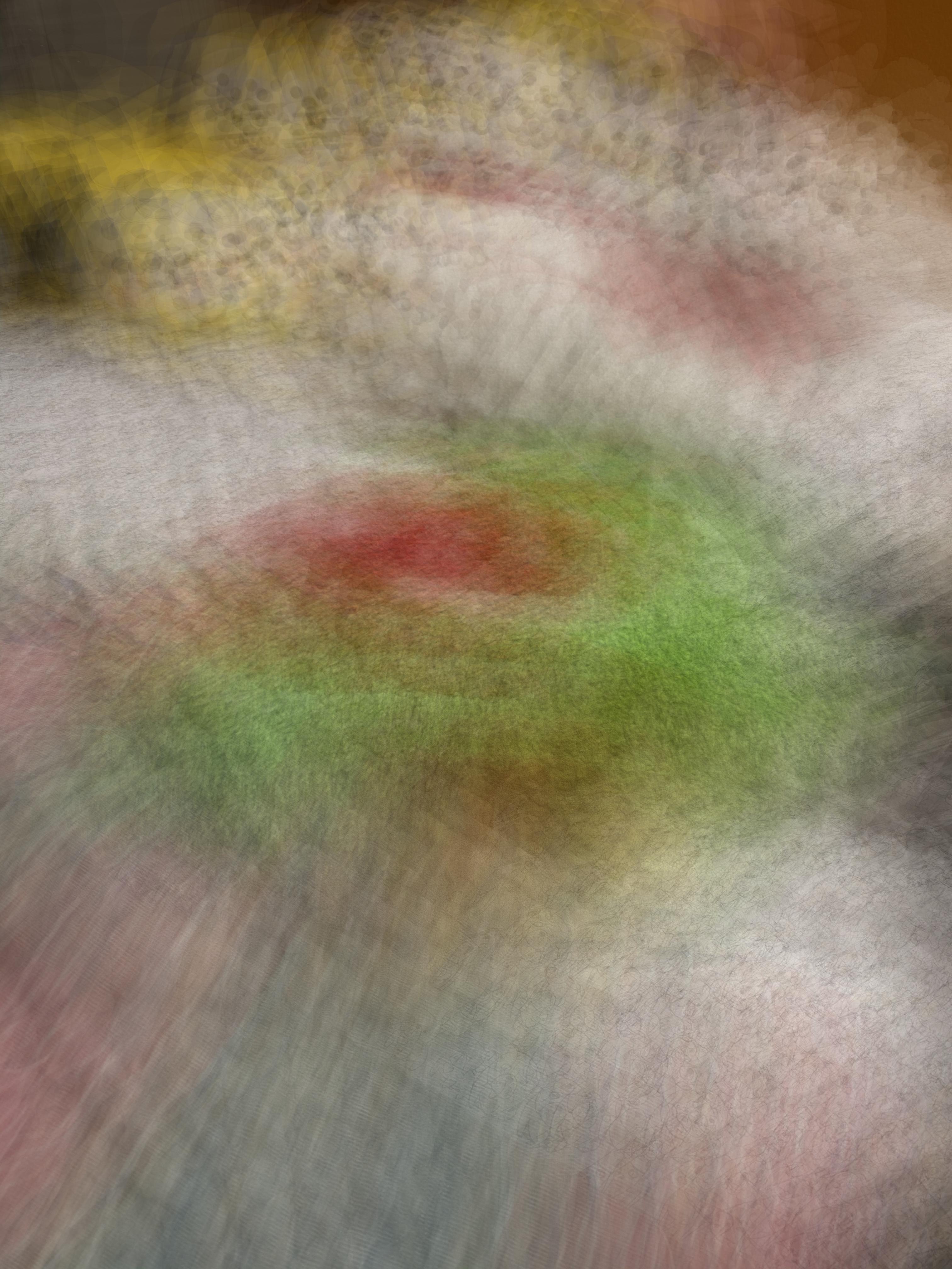
In this section, we attempt to test our code with self taken images in order to see if we can refocus an image using a smaller amount of subaperture images. The given data set uses hundreds of images, but the number of images taken for this section was using 5 x 5 grid, with only 25 images. It is clear that the refocusing did not work, as we can see the images just look blurred. However, it is a nice effect on the images, giving it an almost paint like quality.

It is likely that this set of images failed due to the process of taking images. They were shot on a phone camera, without a tripod, so it is likely that the grid is not consistent in terms of positioning. It is also possible that the grid may be too small and that 5 x 5 may not be enough in order to get a clear image, since there's a lot less images to average. This is apparent in that some of the images are appearing faded in the final result, suggesting that more data may be needed. Overall the thing I learned from this bells and whistles attempt was that taking photos for a lightfield camera is challenging, and it would benefit greatly from using some form of tripod and some standardized way of taking the images so that the grid remains consistent. It would also be helpful to take more images to have more data to work with. However, the resulting images are kind of nice, albeit, unrelated to the project ;)

Project 2: Image Quilting

In this project, we explore different methods of texture stitching using image quilting. We first use a random approach, then attempt to match similar patches to each other and overlap, and then finally, use seam cutting in order to fit patches together. We also use a similar method to do texture transfer, which is done using the same algorithm as texture synthesis, but adding an extra error term to account for when choosing patches.

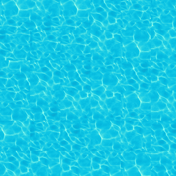
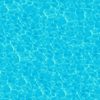
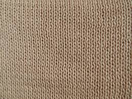
Texture Synthesis

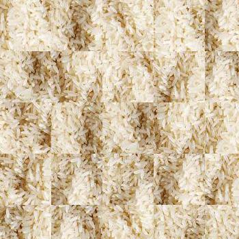
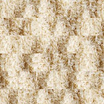
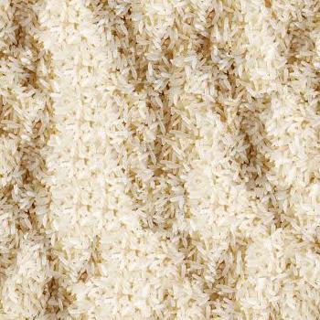
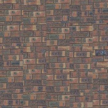
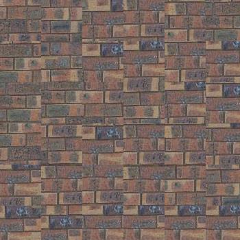
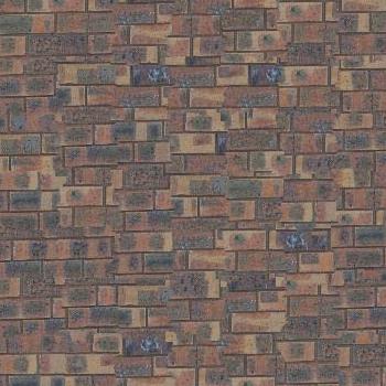
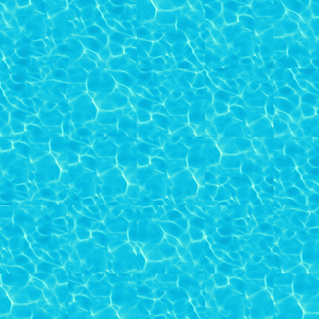
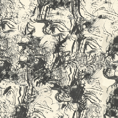
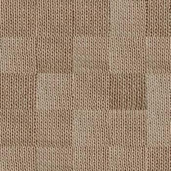
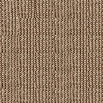
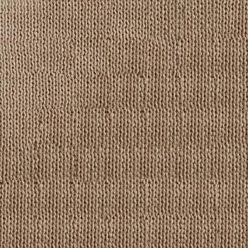
Here we explore 3 different methods of texture synthesis, random sampling, overlapping, and seam cutting. As we can see, random sampling results in strong edges which are very apparent. Overlap improves upon this, as these edges are not as strong, but are noticeable. Seam cutting, reduces these strong edges by fitting the patches together and removing strong artifacts.

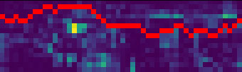
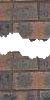
We can see the method used to cut the patches using seam finding to find the mincut. After we find the patch that best fits, by finding the lowest ssd error between the overlap regions, we can perform a mincut on the patches to fit them together and removing the hard edges Here we have two one on the top and one on the bottom. The overlap cost is shown, which is the ssd of the overlapping region between the top patch and the bottom patch. Using the mincut code provided, we find the mincut through this cost to be below, outlined in red. After we find this cut, we can use the returned mask in order to combine the two patches using the mask as a way to stitch the two together. We repeat this until the output image is filled up. In short, the full algorithm is as follows:

1. For the top left patch, randomly choose a patch from the sample texture
2. Then, choose the next patch going from left to right, top to bottom, by using the left and top patch. For every patch in the sample, compute the ssd of the left and top overlap patches. Choose one from the K lowest.
3. After choosing a patch, compute the ssd images between the left and top patches overlaps. Use these ssd images to find the mincut
4. Once the mincut is found, apply the mask to the patches of both the left, top, and chosen patch.
5. Combine the patches

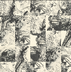
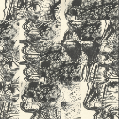
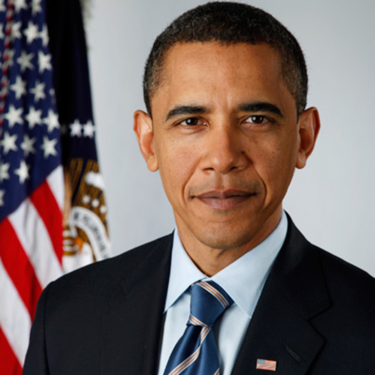
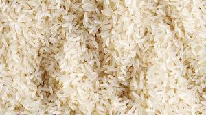
Texture Transfer

In this part, we follow a similar method to texture synthesis, but add in an extra error term to consider when choosing patches from our texture image. In addition to computing the error between the overlap between two patches, we also take into account the error between the chosen patch and the target image's patch in terms of grayscale luminence. Essentially, we are finding how similar our chosen patch is to the place we're trying to fill in the target image. We also use an alpha term, which essentially tells us the tradeoff between the overlap error and the luminence error. Aside from this extra error term we use for choosing patches, we essentially follow the same method as synthesis.

Throughout this part, I had to make some small tweaks that probably weren't done in the paper. The main headache was dealing with finding patches in the target image, since the image won't necessarily be in a size divible by our patchsize. It was a pain to have to calculate smaller patches once we got to the edges of our image. One approach I tried was to pad the target image so it would be divisible by the patchsize, but I realized this would probably lead to some errors since we are using the target image patches to take the ssd between the texture patch. What I ended up doing was a hacky method, which was resize the image to be divisible by the patchsize, then resize the output to be the original image size. This ended up working out since we were still matching the textures, but then resizing them after. I didn't find any grievous errors by doing this, so I kept this method, although I'm sure I could have implemented a method without resizing.