CS 194-26 Final Project

Catherine Lu and Patricia Ouyang, Fall 2020

LightField Camera

Overview

Traditionally in photography, parameters such as focus and aperature size must be set appropriately before taking a picture. If the parameters are off, the picture must be retake or the moment may just be lost.

With a lightfield camera, as designed by Professor Ren Ng, it is possible to adjust the effects of these parameters even after taking a photo. In this project, although we did not have access to a lightfield camera, we used the data from a light field, a series of images taken by cameras placed in a grid orthogonal to the optical axis, to achieve the effects of depth refocusing and aperature adjustment after the images were taken.

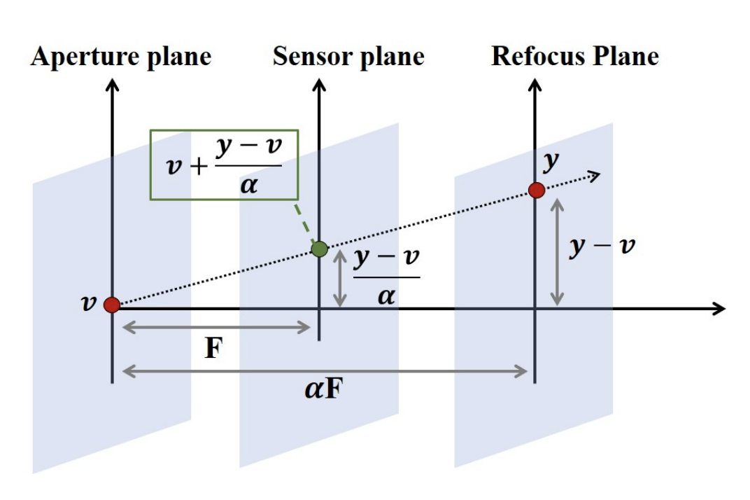
Depth Refocusing

To refocus the image to a different depth, we shifted the images according to the point that we wanted to focus on and averaged all of the images in the lightfield. This gives us the refocused image, because the aligned parts of the images will be in focus while the unaligned parts of the image will result in a blur.

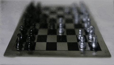
In the gif below, we aligned all the images to the center point of the chess bords and divided the amount shifted by a factor, alpha, relative to the depth we wished to refocus to. Figure 1 from Dayan et. al. 2009 shows that alpha is the ratio between the depth of the original image and the depth that we are refocusing the image to.

Aperature Adjustment

In order adjust the perceived aperature, we aligned the images and then averaged random samples of different sample sizes to get the effect of different aperature sizes. Averaging more images together resulted in effect similar to a large aperature size while a averaging less images together was similar to a small aperature size. This is because with large aperatures, the image has a shallow depth of field, so objects in the background will be very blurry. This is achieved with lightfield data, by averaging more images together which results in a softer background. Thus, averaging less images together will reduce blur, giving the sense of a smaller aperature size.

Augmented Reality

Overview

In this project, we inserted synthetic objects into a video we captured. To do this, we needed to take a video and obtain 30 coordinates for points in the real world that corresponded to points in the video. Using the known points, we calibrated the camera and projected a 3D cube into the scene.

SetUp

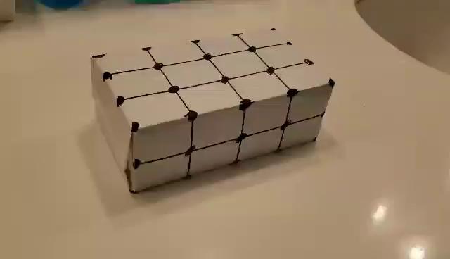
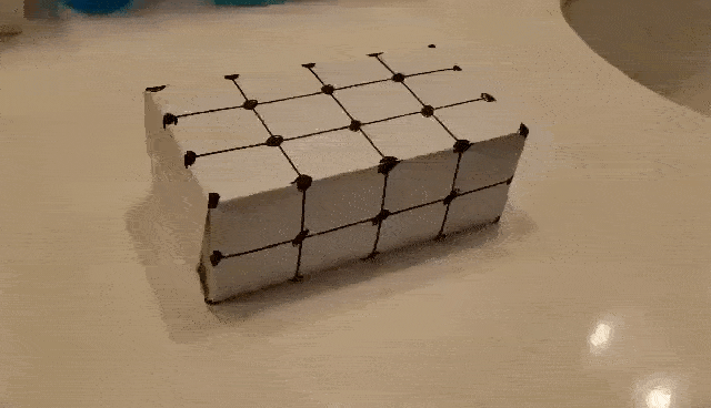
For the setup, marked an even grid on a box as shown in the image above. Then, we took a video of the box, while panning from one side to the other.

Selecting and Propagating Points

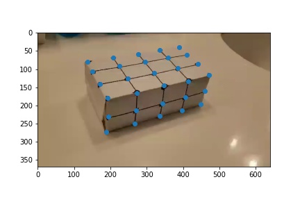
Next, we selected keypoints on the first image of the video so that they correspond to known 3D points in the real world.

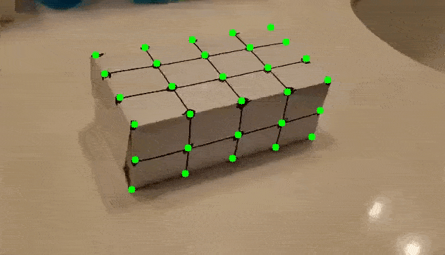
These points are then propagated to the other frames of the video using an OpenCV tracker. We used the median flow tracker in order to obtain these results. The median flow tracker works by comparing the movement of an object in forward and reverse directions in time. Thus, it works well for this application, where there are only small movements of tracked points across frames and the motion is predictable since we are panning across the box.

We encountered some difficulties in utilizing the tracker initially due to having indistinctive keypoints. To remedy this problem, we made a couple of changes including retaking the video on a plain surface as well as clearly marking the points we were tracking. These changes can be seen in the results below.

Calibrating the Camera and Projecting a Cube into the Scene

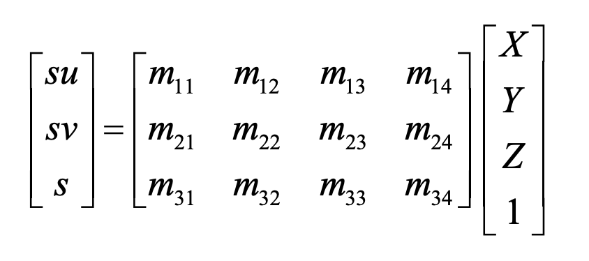
Using the propagated keypoints for each frame, we computed a transformation converting between the 3D world coordinates to the 2D coordinates in the frame. We used least squares to solve for the projection matrix from world to camera coordinates.

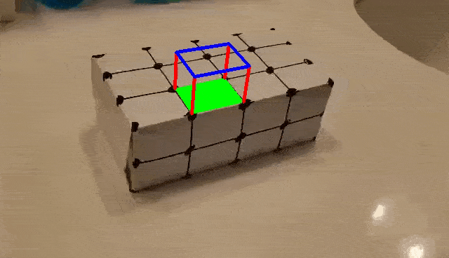
After computing the projectation matrix for each frame, we can project a 3D cube into the image.

CS196-26 Final Project: Image Quilting

Project Overview:

The general goal of this project is to generate quilts of different textures using different methods. Most quilt photos will be grouped together later for comparison purposes.

Randomly Sampled Texture

One way to create a quilt is to just randomly sample patches from the original texture and use them to fill in your final quilt output.

Overlapping Patches

Another way is to randomly sample the first patch of the quilt on the upper left and then fill in subsequent patches by checking which patch in the texture is the most similar (SSD) over some overlapping area between the two and then pasting the newfound patch in next to the previous patch (and over the overlapping patch) until all the patches are filled. If patches are not on the top or left edge the overlapping area includes both the top and left sides of the new patch we're checking.

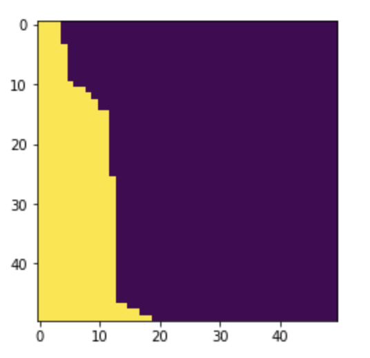
Seam Finding

Finally instead of directly pasting the best patch into the final output each time we can try to find a seam that separates which pixels come from the previous patch(es) and which pixels are filled in from the new patch. This makes it so that the edges aren't so obvious when we paste in the new patch compared to the previous overlapping technique. Getting the seam involves computing a cost matrix that contains the cost associated with having the seam go through each pixel in the overlapping section and then finding the min-cost path through the overlapping section using dynamic programming. We implemented our own min-cost path function in python since the project was not done in matlab. If there are two overlapping regions you can combine the two seam masks (one involves some more transposes) to determine which pixels come from which source. Below is an example of a vertical seam mask found using the function for some patch in the top row of the quilt and the two overlapping regions the seam mask is for.

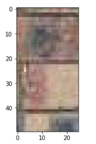
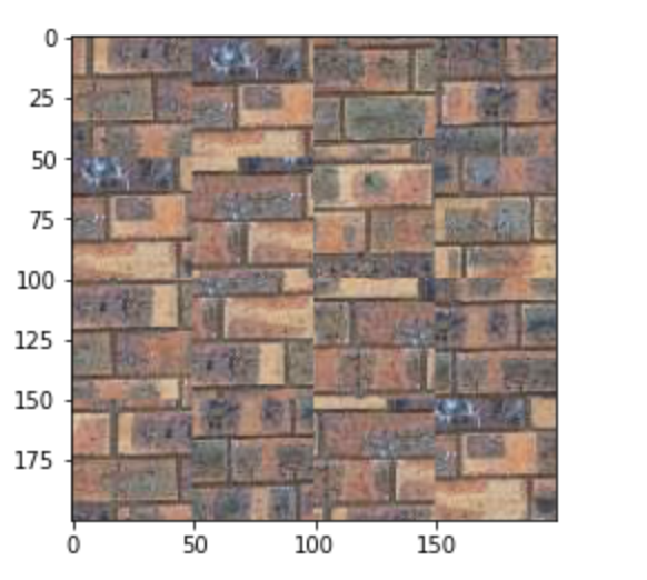
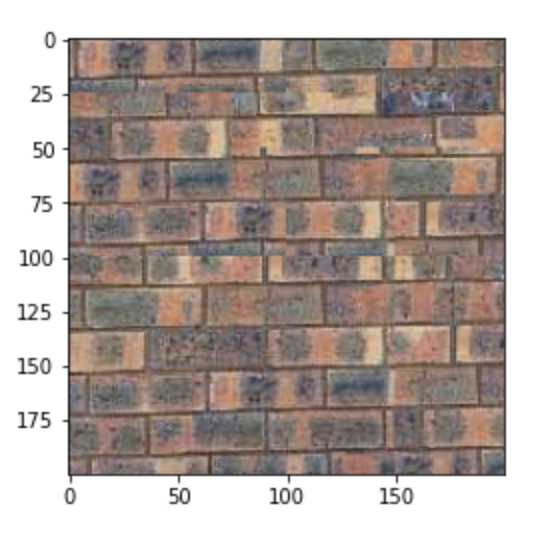
This is the right vertical overlapping region of the brick on the left.

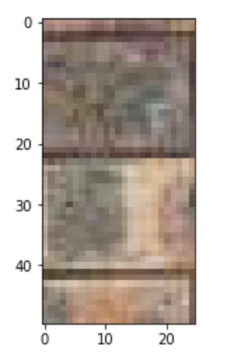
This is the left vertical overlapping region of the new brick on the right.

Quilt Comparisons

Quilt order: Original phot and randomly sampled, then overlapping patches and seam finding.

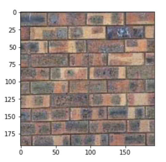
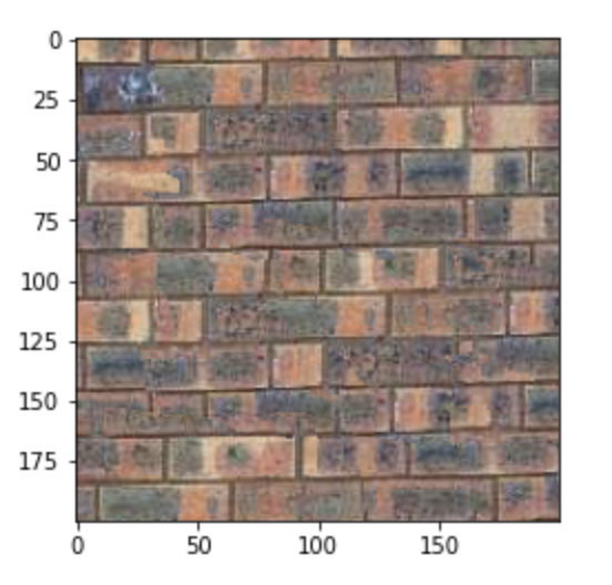
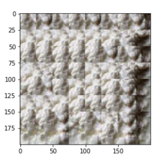
Bricks:

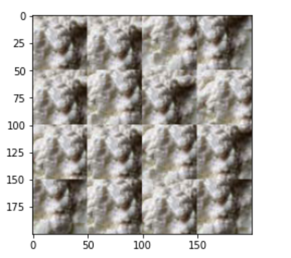
Yogurt:

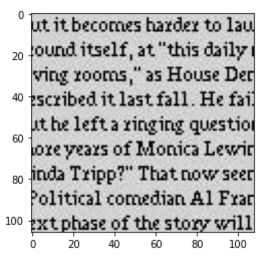
Text:

Additional seam quilt examples using other textures:

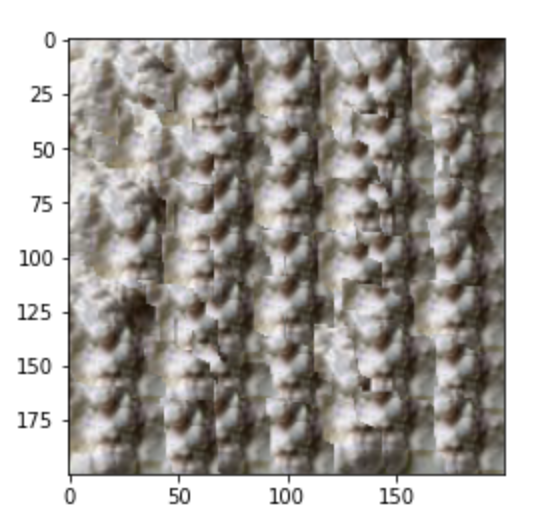
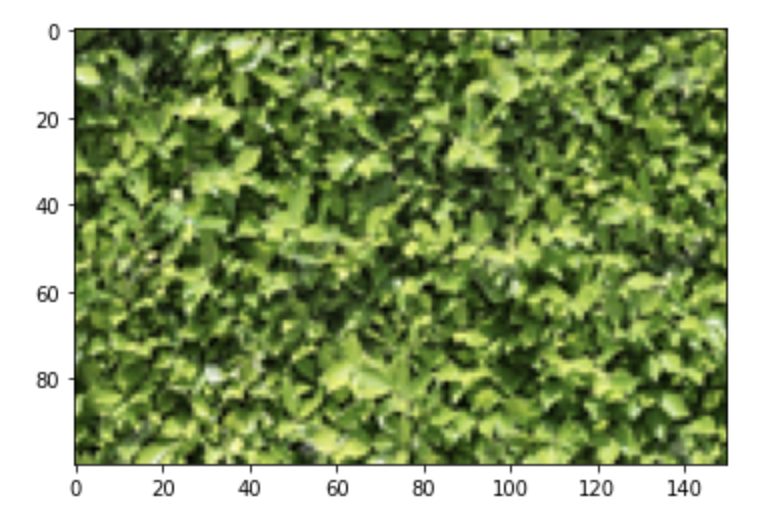
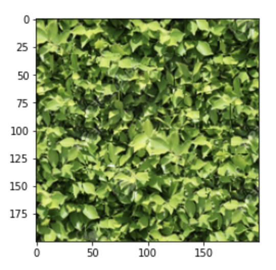
Hedge:

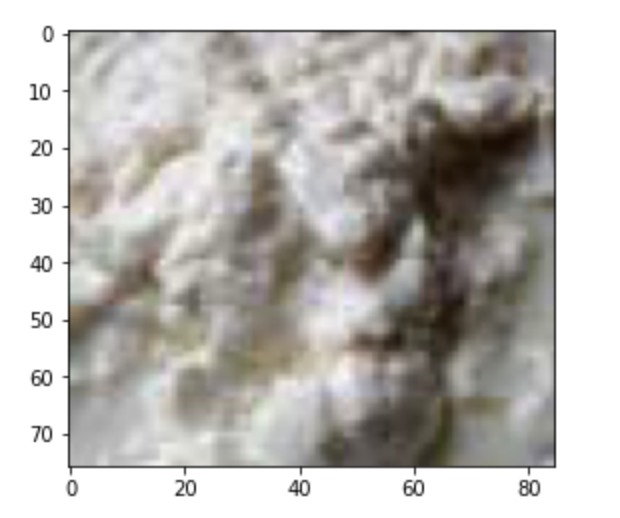
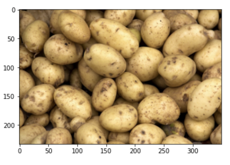
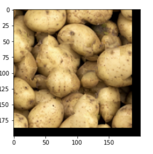
Potatoes:

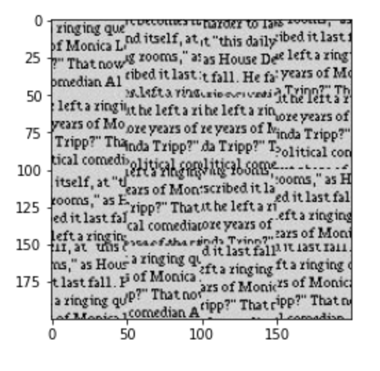
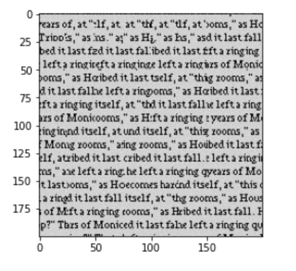
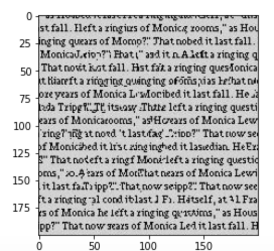
Texture Synthesis

Now we can create new versions of images that are sampled from some texture. This involves modifying the previous seam-finding technique such that the new patches are chosen not only based on the SSD but also some other factor to maintain the target image shape. In this case I turned the target image and texture image into grayscale and computed the difference for the additional cost value.

Bells and Whistles

We implemented our own cut function in python for seam finding. See code submission for details.