The model I ended up using is a pretrained VGG net. The net I chose has a total of 36 layers, and uses MaxPool2d for its pooling layers. However, at the suggestion of the paper, I replaced the MaxPool2d layers with AvgPool2d layers. (The improvement in model performance will be demonstrated below). Additionally, I changed the ReLU layers to no longer being computed inplace (although this distinction is much less relevant than the prior distinction). In terms of hyperparameters, I ultimately settled upon using a relatively high learning rate of 0.001; I chose this because I noticed that having a lower learning rate was not beneficial to model performance and, in fact, generally meant that I required more epochs to achieve similar results. I additionally added a non-zero weight decay hyperparameter. On some inputs, this made a slight difference. I ultimately could not identify the exact impact of adding a weight decay, but I settled upon a 0.001 weight decay.
There some key differences between the model I used and the model used in the paper. Firstly, the paper uses a 19-layer model (whereas the pretrained VGG net has 36 layers). I did not experiment heavily with the number of layers; but I chose the specific VGG net because it appeared to do the job well enough. Secondly, as mentioned above, I changed the pooling layers. Thirdly, the paper performs its content and style constructions upon various Conv2d layers inside the network; through some experimentation I noticed that I can occasionally achieve slightly more appealing results when I perform the loss calculations and constructions upon ReLU layers. I don't actually know why this is the case and I suspect there is minimal difference. Finally, I chose 1000 epochs as my go-to number of epochs: this seemed to work the best and going beyond this didn't help image quality.
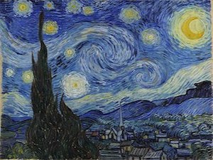
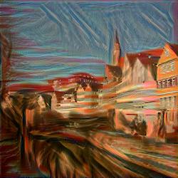
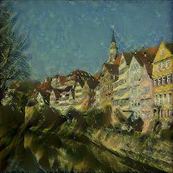
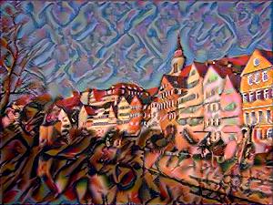
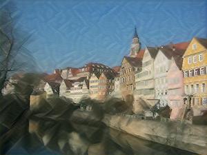
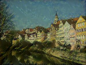
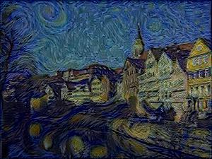
Firstly, here is the original Neckarfront image and after it, the five style images used in the paper. Note that the original aspect ratios of the style images are not necessarily preserved here.

Before I display the transfer of the various styles in the paper to the Neckarfront image, I will display some interesting intermediate results.
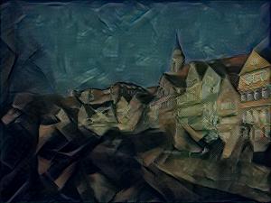
I mentioned earlier that I used the AvgPool2d instead of MaxPool2d; here are some examples of the difference in quality (run with the same number of epochs). In each of the below image pairs, the left image used max pooling while the right image used avg pooling. Note that the images are square here (for simplicity's sake during initial testing when I was coding the project).
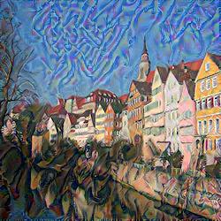
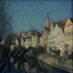
The most distinct effect of using average pooling is that the colors from the style image are transferred over better; moreover, the textures are more pronounced and more evident.
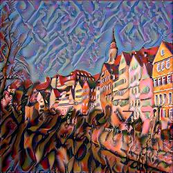
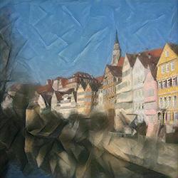
The number of epochs made a substantial difference as well. Below, for each set of images, the leftmost image is constructed with only 100 epochs, the middle image uses 500 epochs, and the rightmost image uses 1000 epochs.
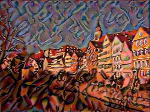

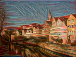
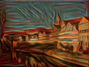
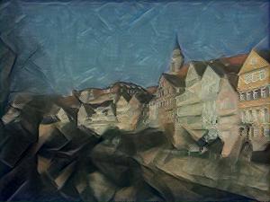
As you can see, having too few epochs meant that the output images looked mostly like the content image with only a little bit of distortion indicating anything had changed about the image.
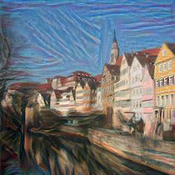
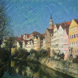
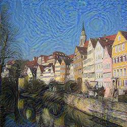
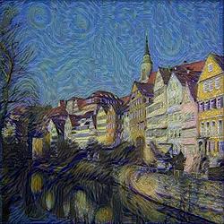
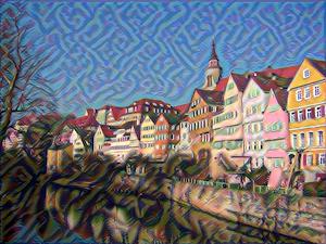
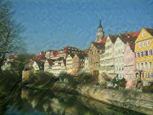
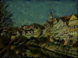
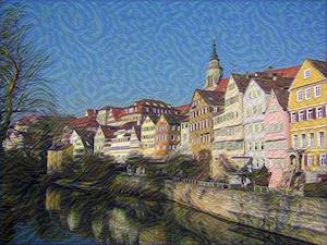
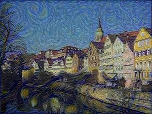
Alongside the initial Neckarfront image, here are the final results (the rightmost column from the images above):
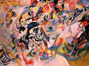
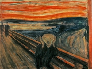
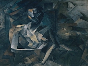
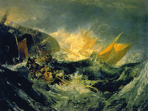
Without further ado, here are the results of transfering some styles I have selected onto a content image of my choice.
Here is the content image (top left) followed by the style images.


Here are the results.
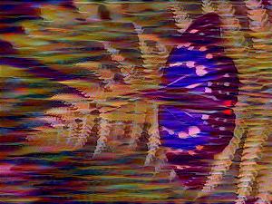
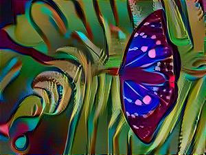
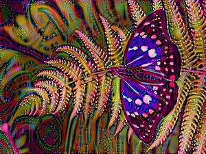
As you can see, the bottom two images appear to have the style successfully transfered, but the top right image seems to have done poorly. My understanding is that the boat image seems to have the predominant characteristic of being "smudged" horizontally; that is, I had intended for the "flaky" oil effect on the boat painting to be transfered, but what was transferred instead was the horizontal nature of the image instead. This results in a butterfly image that appears horizontally smudged, rather than actually looking like the original image.
I provide credit to various online sources that assisted me in the implementation of different phases of this project, including the original paper as well as resources that helped me understand neural network structure and implementation. These include:
https://towardsdatascience.com/this-thing-called-weight-decay-a7cd4bcfccab?gi=c8cd5c1d737
https://arxiv.org/pdf/1508.06576.pdf
https://stats.stackexchange.com/questions/315626/the-reason-of-superiority-of-limited-memory-bfgs-over-adam-solver
https://pytorch.org/hub/pytorch_vision_vgg/
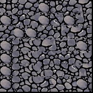
For this project, I used the provided sample textures.

Additionally, I added two sample textures of my own choosing.
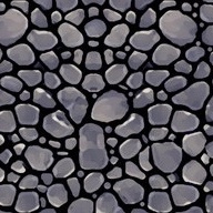

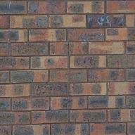
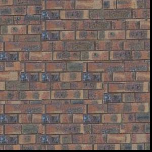
For this portion, I merely obtained random samples from the sample image and slapped them together as specified. Here is an example of an output generated by randomly sampling from the bricks_small texture.
The image is 300x300, and each sampled patch is 50x50. The image is noticably "blocky" and does not seem very realistic. This is because randomly sampling patches means that there is a high likelihood that patches that ended up adjacent to each other in the output don't make real-life sense next to each other (whether it be the wrong coloration or the wrong alignment of edges/features in the patches).
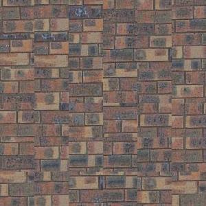
For this task, I implemented ssd_patch and choose_sample more or less as suggested in the project spec. Below, I include several examples with varying tolerances. From left to right, the tolerances are: 0.00001, 0.01, and 0.1. I ultimately selected the 0.1 tolerance as suggested in the paper.
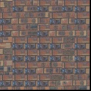
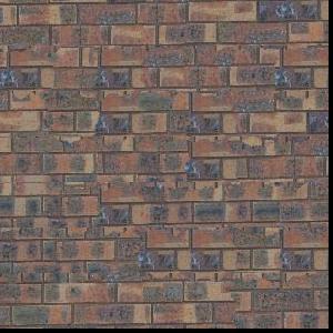
Below, I've included the Randomly Sampled Texture output on the left and the Overlapping Patches output on the right for some quick comparison of the quality of the texture synthesis.
As is immediately obvious, the overlapping version on the right is much more realistic and is much less "blocky" than the pure random version on the left. This improvement over the purely random approach comes from the overlapping sections, where we deliberately address the problem mentioned earlier of adjacent patches not aligning in color or edges/features. While we don't explicitly look for edges/features in this section, computing a SSD helps moderately in this regard.
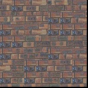
Here are five of the results that I produced. The top three are from the provided sample textures; the bottom two are from my own selected textures.
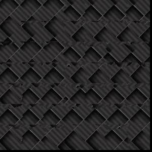
The results aren't amazing, admittedly. I didn't have enough time to realy figure out how to fix them, but an observation I made during this was that vertical seams appeared to be handled worse than horizontal seams. I cannot figure out why this would be the case; however, I'm guessing that my implementation of computing the vertical seams or otherwise combining the horizontal and vertical cut masks is flawed somewhere.
I unfortunately did not have time to implement this section.
As I was working in Python, I naturally could not use the cut.m provided in the spec. Moreover, I am not familiar with matlab and could not even begin to read cut.m. So, I implemented my own version of cut which can be found in quilt.py and all images generated for the Seam Finding portion use my own version of cut.m.