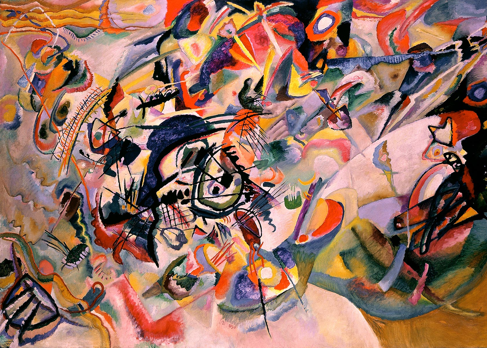
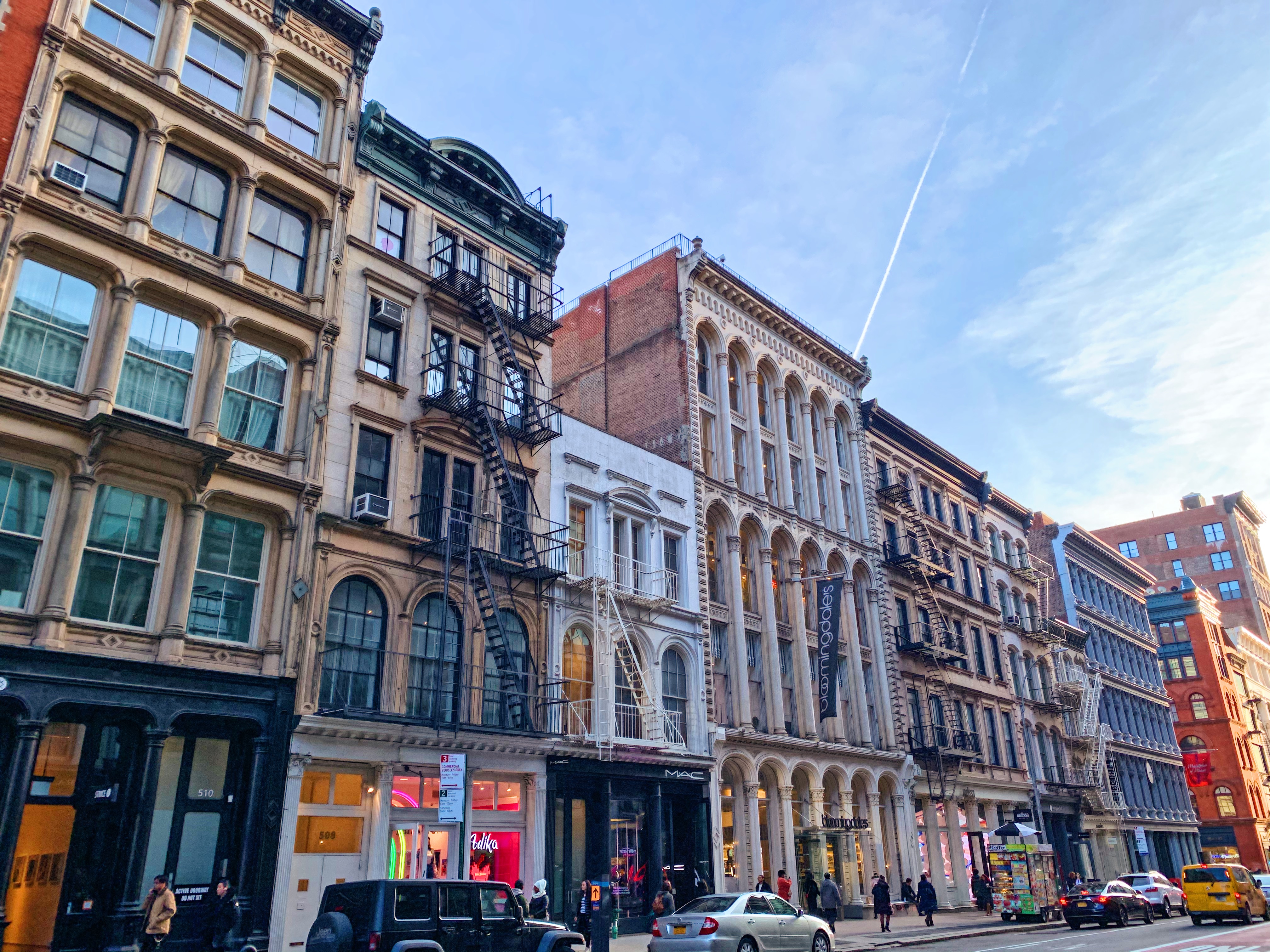
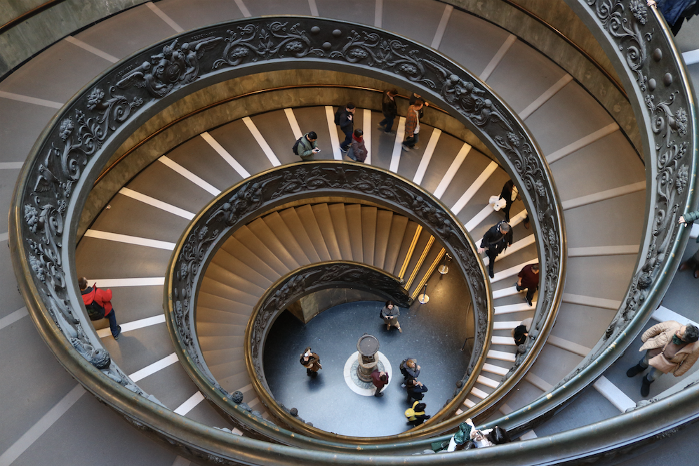
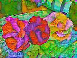
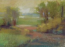
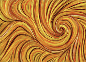
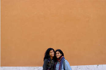
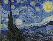
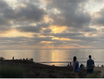
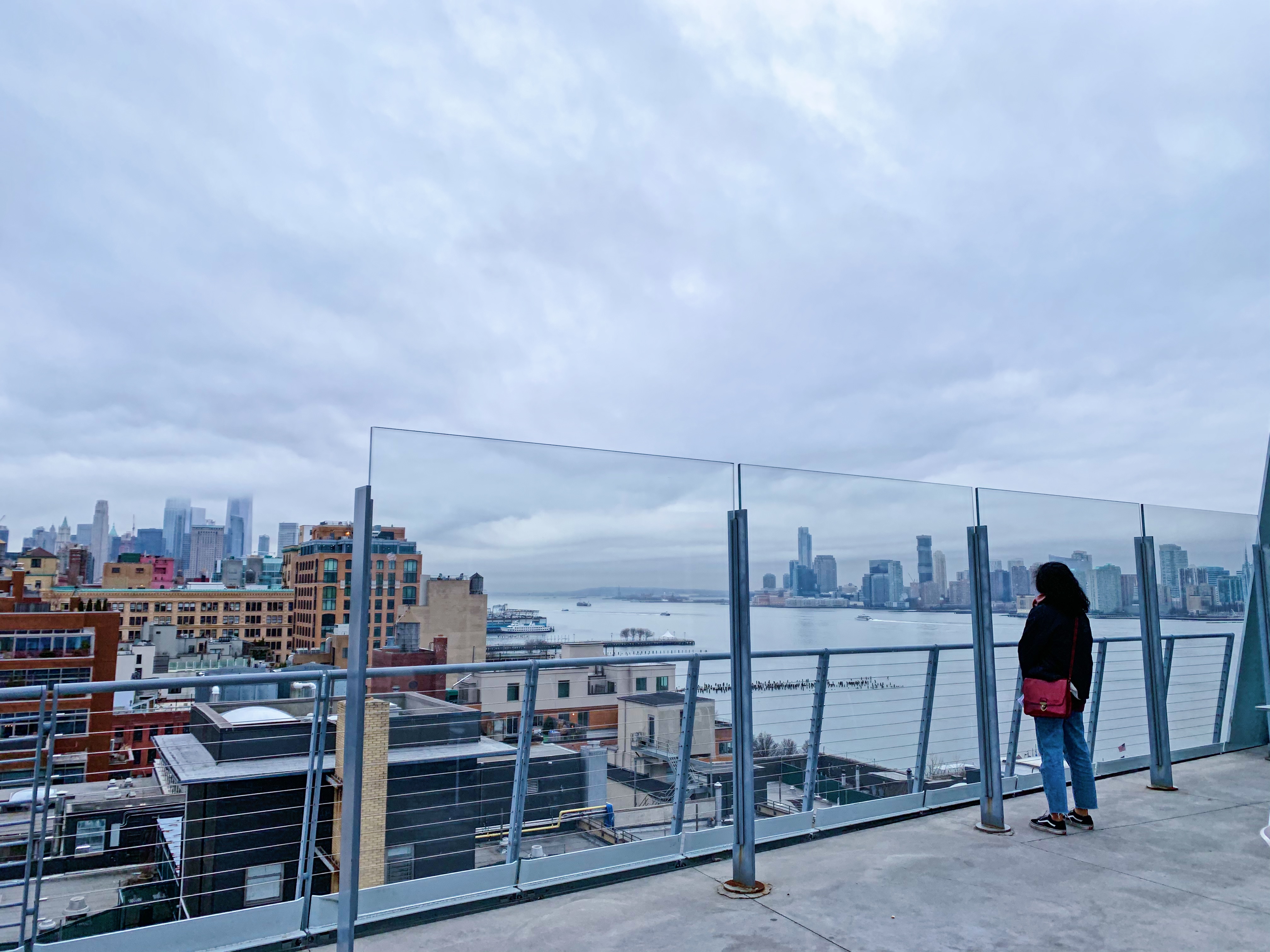
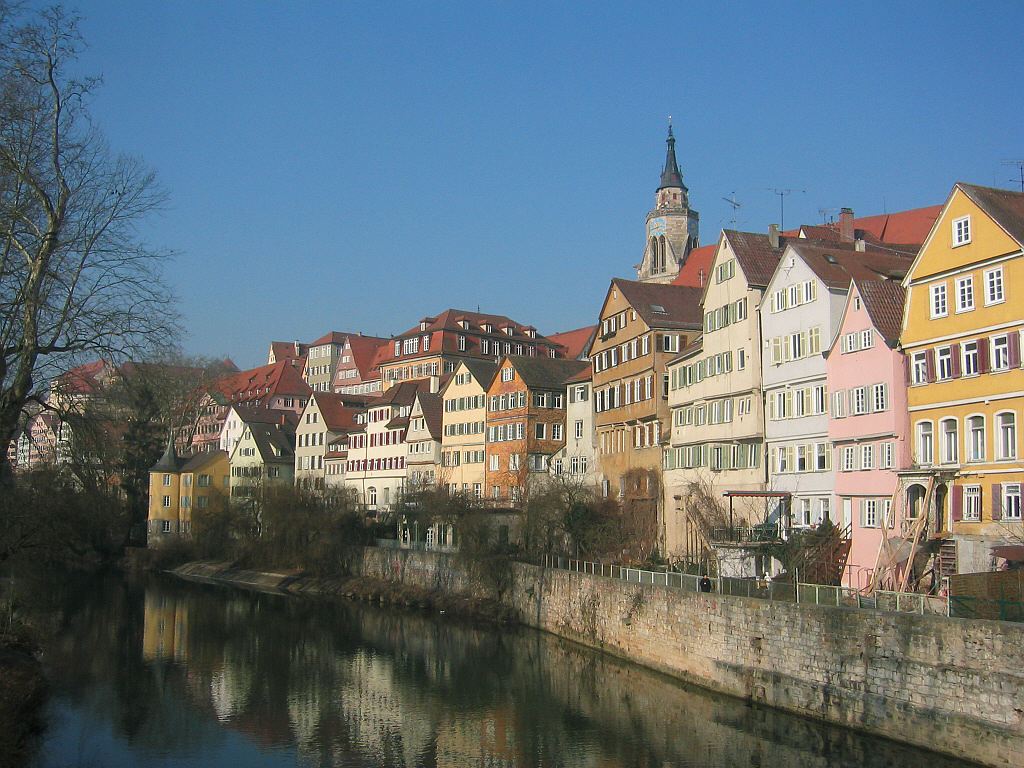
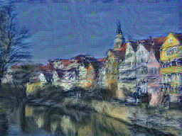
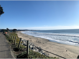
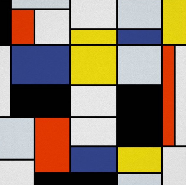
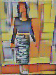
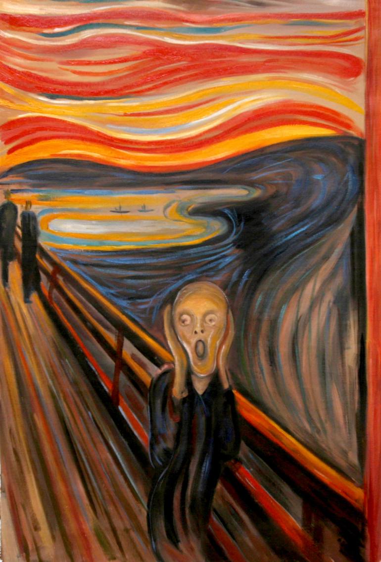
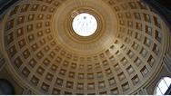
This neural style transfer project is hands down my favorite from this semester. This project is based on this paper by Leon A. Gatys, Alex S. Ecker and Matthias Bethge. The goal of this project is to take a pattern image or painting and transfer its style onto a content image (a photograph).
In order to do this, we work with deep neural networks. One of the main takeaways of this project is the idea that neural nets are extremely strong tools, particularly with their power to separate content from style within images. The paper explains how we can use an artificial system that uses neural representations and reconstruct the content and styles of different images.
As the paper states, “The system uses neural representations to separate and recombine content and style of arbitrary images, providing a neural algorithm for the creation of artistic images. Content refers to the actual pixel values in an image. Style refers to a higher level overall architecture of an image.”
At a high level, the algorithm described in the paper independently separates the content and style of each image (does this using a neural network). As we delve into further convolutional layers of the network, only the higher level features are kept, so the reconstructions of the image include less detail.
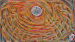
To get more specific, I used features from the pretrained VGG_19 batchnormed model, as specified in the paper, to extract low level features from the images. The algorithm initially begins with a random noise image. Then, we use gradient descent to create a resulting image. We reconstruct an image's content and its style from various layers in the neural network.
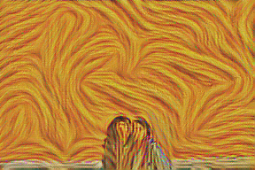
Once content and style features are extracted, we compute our total loss. The function is a weighted sume of two components: the style loss and the content loss. The weights indicate whether the resulting image leans towards the content or style.
This is measured by squared-error loss between the feature representations output and input image. Essentially, it indicates how the feature map of the result image differs from the feature map of the source image. As described in the paper, we match the content representation on layer conv4_2.
For style loss, the layers we are interested in are CNN1_1, CNN2_1, CNN3_1, CNN4_1 and CNN5_1 as described in the paper. The style loss is a bit different than content loss because we don’t want style loss to include regional information. Because of this, we use the Gram matrices of the feature maps at each layer. We want to calculate the Gram matrix for the feature map of both the content and style image. The style loss is the weighted Euclidean distance between the two Gram matrices. To get the total style loss, we sum across all layers.
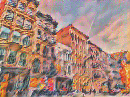
Once we have the style and content loss, we can define our total loss function which is dependent on weighted hyperparameters α and β. The final loss function indicates how much content or style we would like to see in our resulting image. For example, a lower ratio of α / β would highlight style features more.
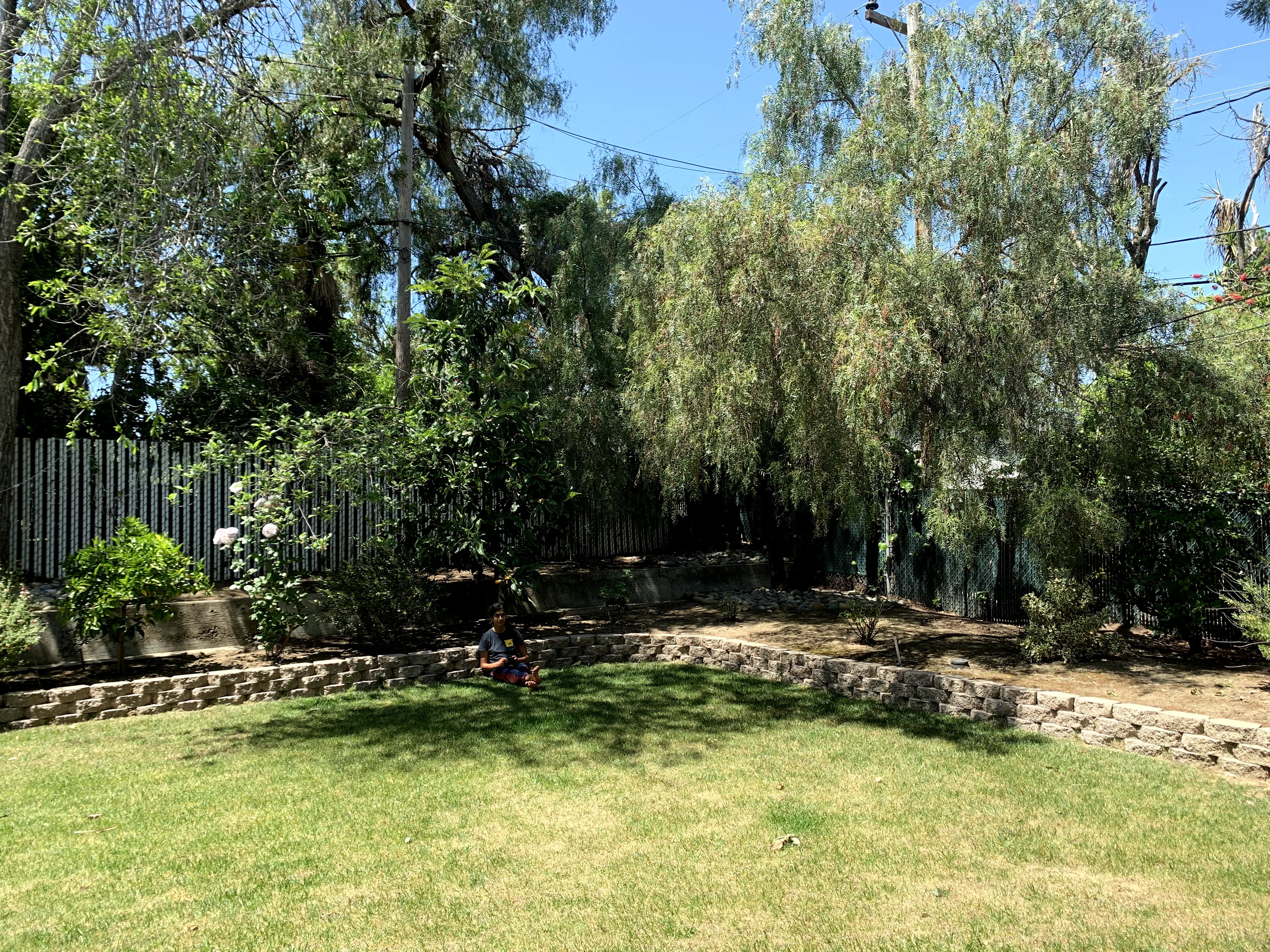
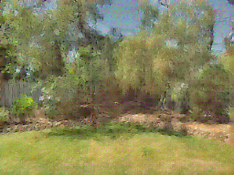
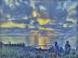
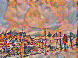
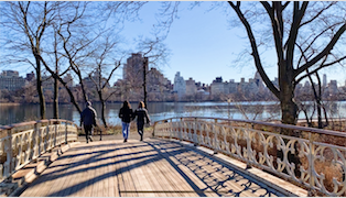
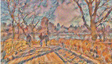
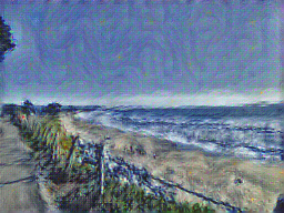
I learned how neural networks can be used for their perceptual abilities within the convolutional layers. These neural networks are powerful enough to separate content and style within images. This style transfer project was definitely one of my favorite in the class because I love taking photos and appreciate art, so I definitely want to continue to use my code to play around with photos I take in the future to create cool looking digital art.
In this project, we are working with light field data. We capture light field data by taking many photographs over a plane orthogonal to the optical axis. Using this light field data, we can simulate refocusing depth and adjusting aperture.
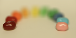
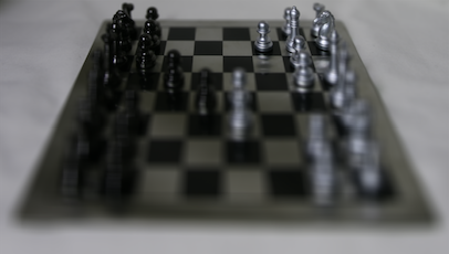
The light field data I used was the Stanford Light Field archive’s light field dataset. This was given in the form of 17x17 grid of images.
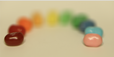
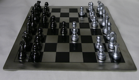
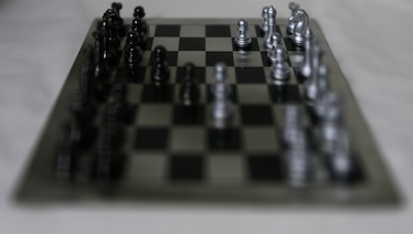
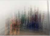
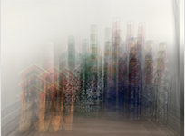
To begin with, I averaged all the images. The initial focal point for the jellybean dataset was on the front objects (the front jellybeans were sharper than the background jellybeans). This was because in the jellybean dataset, the objects that moved the most across the images were the background jellybeans whereas the front jellybeans stay relatively in the same region. For the average of the chess dataset, however, the front chess pieces are blurrier because those objects move around more than chess pieces farther away. Here is the result from this:
In order to refocus the depth, we iterate through all the images and shift them to the center image in the grid. In this case, the center image would be the image at position (8,8). For example, if we are looking at the (i,j)the image, the shift to the center image would be
shift = (i-8, j-8)* alpha where alpha is some constant. Once we shift for every image (using np.roll), we average all the shifted images, which creates a resulting image to focus at certain parts of the image.
Finally, we iterate over a range of alpha values to create an animation of the images focused at different depths. Below are the results:
In this part, we could adjust the aperture of the images. First, let’s define what aperture is. Aperture is defined as the measure of how big the opening that allows light in is. Therefore the smaller the aperture, the less light that is let in, which allows it to focus better on specific parts of the image and hence, the image is sharper. On the other hand, larger aperture means you’ll get a blurrier image. In terms of our grid of images, a smaller aperture is represented by letting in less light and therefore averaging less images together.
In order to simulate changing the aperture while maintaining a constant point of focus, we could take the average of a given radius of images around the center image in the grid (a grid around the center image of size radius * radius). The smaller the radius simulates a smaller aperture because it’ll be more focused.

Finally, we can create an animation of different aperatures by passing in various radii to create images with different aperature sizes. Here is the result of the jellybean data with radius 0-8:
For this part, I uploaded my own grid of images (attempted to create lightfield data) and used my refocusing function on this data. As you can see from the result below, it didn’t end up refocusing very well. I captured 16 photos in a 4x4 grid of a set of rocks in a U-shape (very similar to the jellybean setup). Each individual refocused image itself appeared to be very blurry. This is most likely due to the fact that I manually took the grid of images myself and the fact that there is significantly less data. In the Stanford lightfield datasets, there were 289 total images and in mine, there were 16 total images. Moreover, the spacing between each image probably left a lot of gaps and were too inconsistent as compared to more legitimate lightfield camera data. Because of these reasons, when you try to shift every image in the grid to the center and average all of them, the objects in the image don’t align well and the objects end up appearing in different positions in the resulting refocused image.

With this project, I learned a lot of very applicable lessons, especially for phototaking itself. One of the biggest things I learned is that with a lightfield camera, you can simulate many different image processing strategies. This is because lightfield cameras provide a lot of data, where only shifting the position of various images is required to achieve a certain effect (like refocusing or aperture). Moreover, I take a lot of photographs in my freetime. Personally, when I’m taking photos on my DSLR, I end up retaking a lot of my pictures in order to shift certain factors on the camera like focus depth or aperture. Instead of this traditional method of photography, lightfield data changes the way people approach photography because they do not need to retake many photos and later edit additional features on their computer. If you have enough lightfield data, you can achieve the adjustment of aperture and depth refocusing through code similar to what I implemented above.
