Data Preprocessing
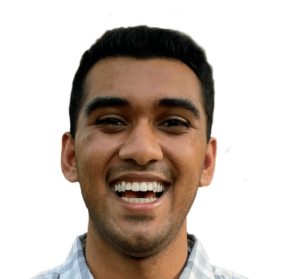
In this part, I did some simple image preprocessing to read in the images and transform them before feeding them into the model. Namely, the preprocessing consisted of:
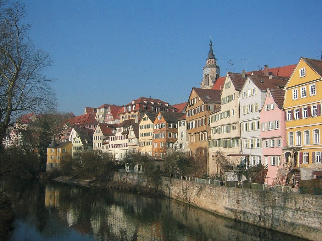
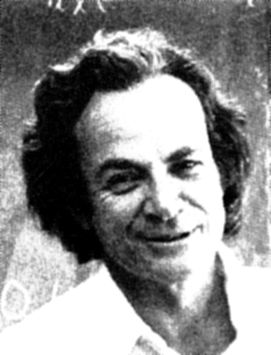
Above, you see the original image that we will be applying various art styles to. Those styles are highlighted in the artworks below:
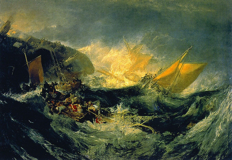
The Shipwreck of the Minotaur
J.M.W. Turner
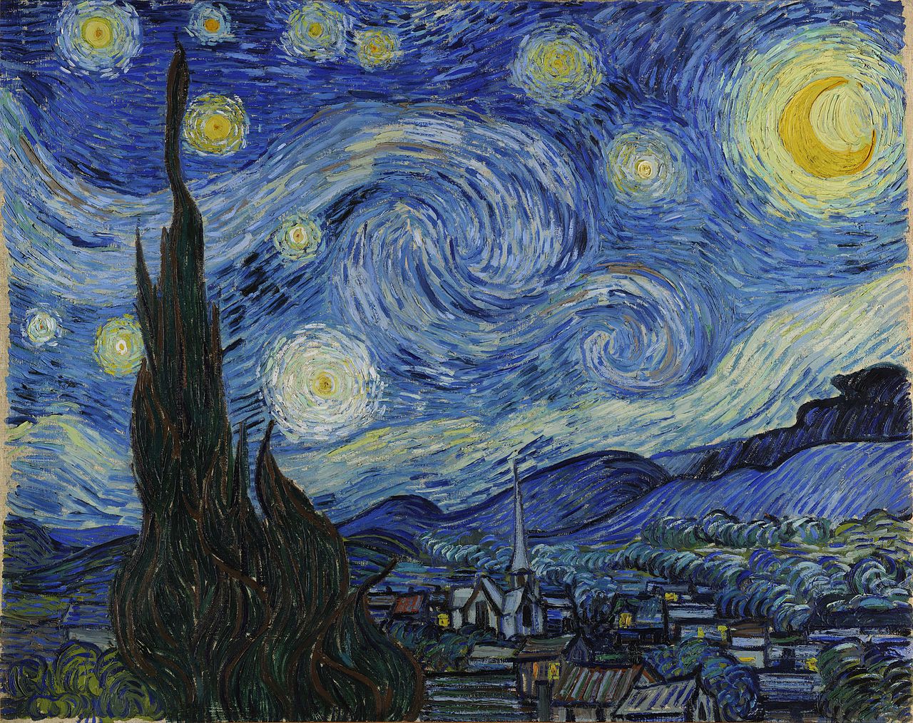
Starry Night
Vincent Van Gogh
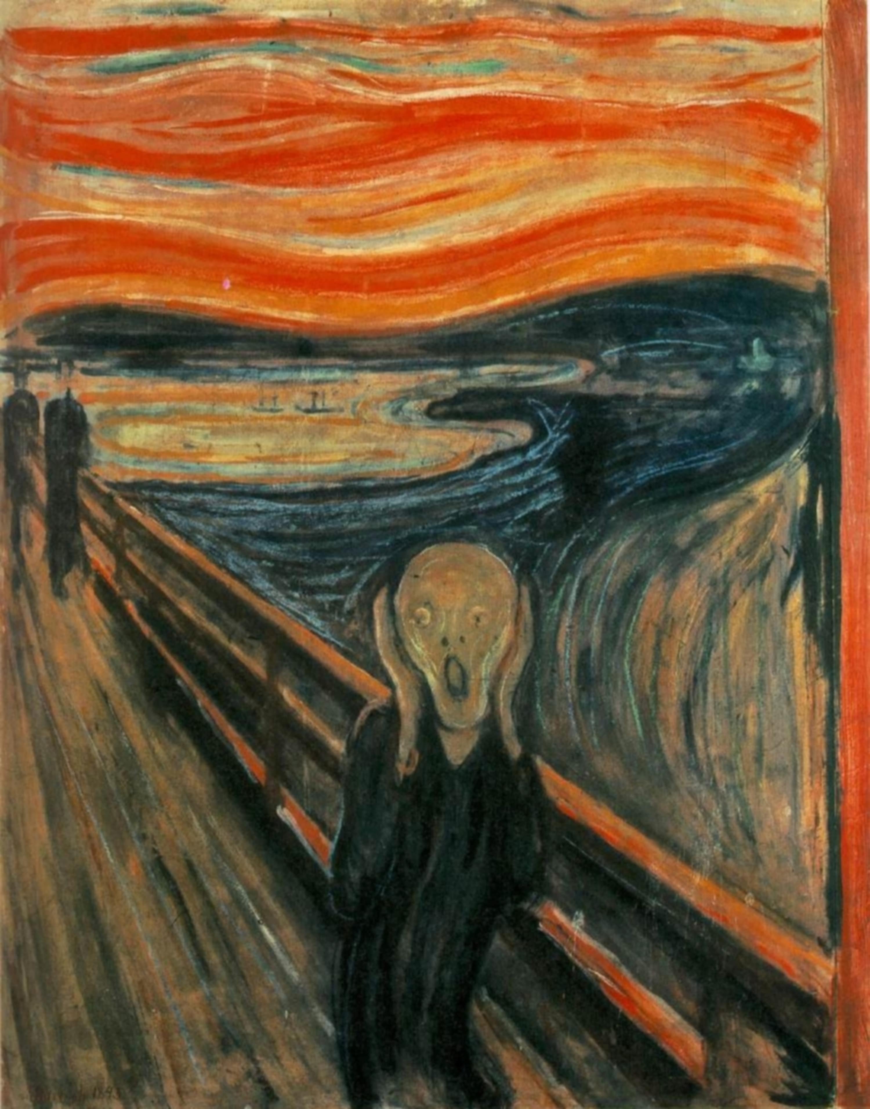
Der Schrei (The Scream)
Edvard Munch
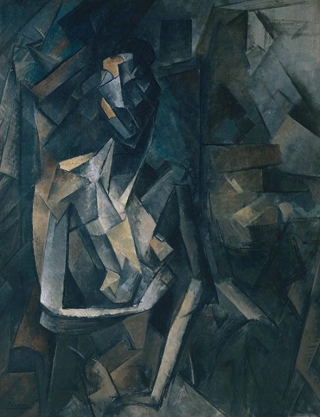
Femme Nue Assise
Pablo Picasso
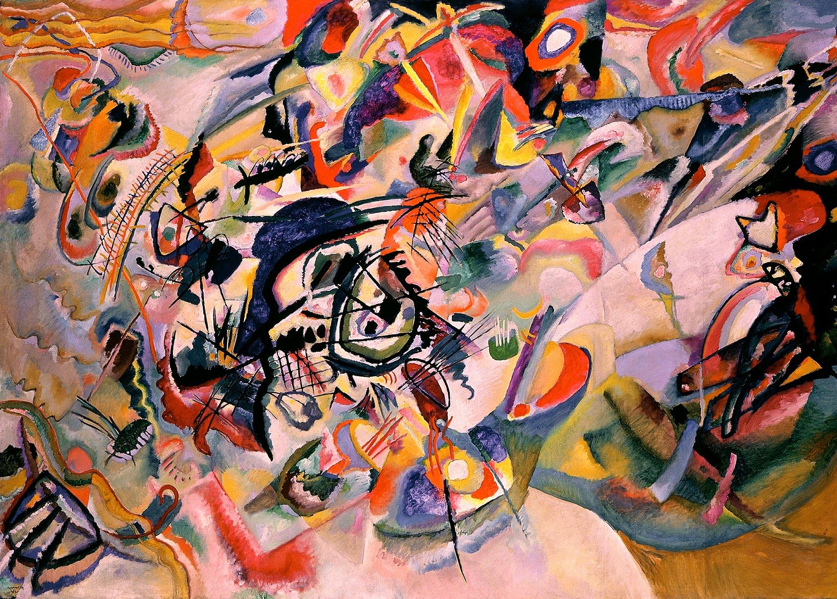
Composition VII
Wassily Kandinsky
CNN Model Architecture
Instead of creating a CNN from scratch, I made use of a pre-trained VGG-19 model (as per the Gatys, Ecker & Bethge paper - A Neural Algorithm of Artistic Style.
Following that paper, I replaced all the MaxPooling with AvgPooling to improve the gradient flow and better the final quality of the image.
In addition, I removed all the fully-connected layers such that there were only convolutional and pooling layers.
Now, for the unique insights from the paper. The paper takes advantage of two key pieces of information that are derived from different stages
of the CNN. Namely, content & style reconstructions.
Content Loss
The content reconstruction attempts to reconstruct the input image from the convolutional layers. The reconstruction from the lower levels is almost perfect, while more detailed (pixel-specific) information is lost in the higher levels. Each layer has N distinct filters with N feauture maps, each of size M (where M = h*w of the feature map). Thus, we can define a matrix F such that F[i,j] represents the activation of the ith filter at position j in a specific layer. We can construct this feature representation for both the original photo (P) and the generated photo (F). As part of this construction, we attempt to minimize the squared error loss between the F and P matrices. This leads to a new component in the neural network that needs to be included after relevant convolutional layers - the Content Loss.The paper only highlights the fourth convolutional layer as the layer at which we compute the content loss. However, I found that applying the content loss at convolutional layers 3, 4, and 5 yielded the best results.
Style Loss
The style reconstruction attempts to build a new feature space that captures the image style on top of the CNN representation. The style representation computes correlations between different features at different convolutional layers of the CNN. The feature correlations are given by a Gram matrix G of size NxN. G can be calculated by taking the inner product of the vectorized feature maps.Now, to generate the texture that matches the style of the image I used Gradient Descent on the original image. This is done by minimizing the mean squared distance between entries of the Gram matrix from the original style representation A and the Gram matrix of the generated style representation G - the Style Loss.
The paper highlighted all the subsets of the 5 convolutional layers as layers on which to compute the style loss. By trial-and-error, I found that applying the style loss after all the convolutional layers yielded the best results.
Personal Touches
In summary, the modification made to the basic VGG-19 model are the addition of the Content Loss and Style Loss layers after the specified convolutional layers and the replacement of the MaxPool pooling layers with AvgPool pooling. As I was researching the VGG-19 model to better understand how it worked, I realized that the pre-trained VGG-19 model is trained on images where it normalizes images with the following means and standard deviations: mean=[0.485, 0.456, 0.406] & std_dev=[0.229, 0.224, 0.225]. In an attempt to standardize this normalization procedure, I added an additional layer to the network that normalizes the new input images in this same manner. Finally, as I was making these changes to the network, I realized that after I'd added all the Content and Style Loss layers, I didn't need anymore convolutional or pooling layers. So, to reduce the complexity and size of the model, I removed all the subsequent layers to yield the final model architecture shown below: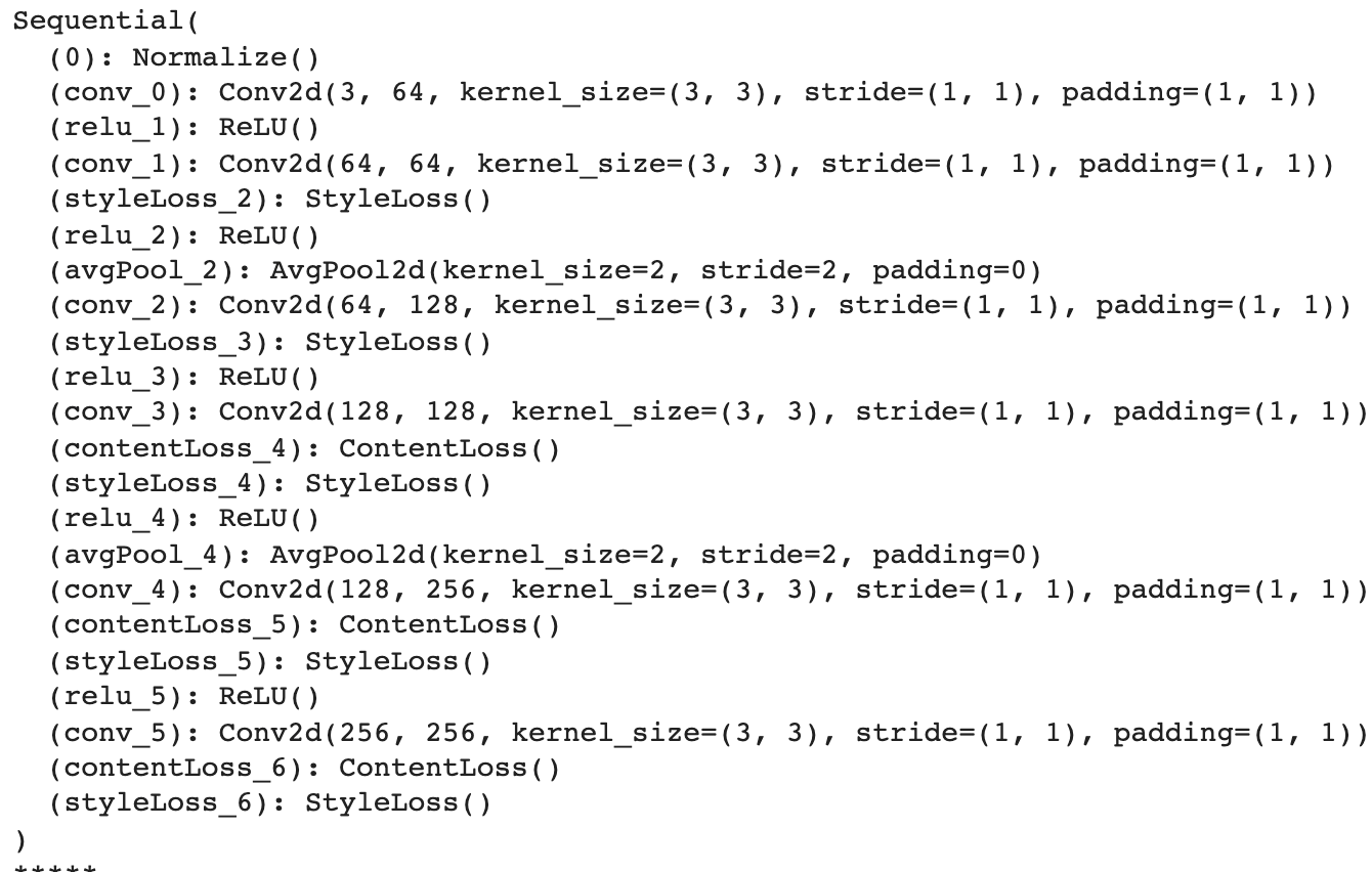
Model Outputs
To make a visually appealing final output, you need to find a good balance between a strong emphasis on style vs content. If you emphasize style too much, you will get an image that matches the appearance of the artwork
(essentially yielding a texturized version of it). But, at the cost of hardly showing the photograph's contents. On the other hand, if you emphasize content too much, you can clearly identify the photograph but the style
of the painting won't be well matched. This tradeoff is highlighted in Figure 3 of the paper, I used the figure to determine the values of alpha and beta in the loss function that combine the Content and Style Loss.
This loss function is minimized during the image synthesis and is a weighted sum of the Content and Style losses where alpha is the weight on Content and beta on Style loss. One key point to note is that there is an additional
weight term associated with the Style loss - it is set equal to 1/5 for active style layers (those with nonzero weight).
There weren't too many hyperparameters that needed to be tuned for the model. The ones that needed to be tuned were the number of iterations and alpha/beta ratio.
The paper suggested running the model for 1000 iterations, but I noticed that the loss function converged before then and that running the model for 300 iterations led to sufficient results. The alpha/beta ratio required some
additional tuning, so I used Figure 3 from the paper as a guide for this. I started with an alpha/beta ratio of 1e-8 because smalller ratios didn't apply enough of the style to the photograph, and increased it to 1e-12. Increasing
the ratio beyond this made it difficult to discern the contents of the photograph. The results are highlighted below:
Neckarfront in Tubingen, Germany x The Shipwreck of the Minotaur
-min.png)
Alpha/Beta Ratio: 1e-8
-min.png)
Alpha/Beta Ratio: 1e-10
-min.png)
Alpha/Beta Ratio: 1e-12
Neckarfront in Tubingen, Germany x Starry Night
-min.png)
Alpha/Beta Ratio: 1e-8
-min.png)
Alpha/Beta Ratio: 1e-10
-min.png)
Alpha/Beta Ratio: 1e-12
Neckarfront in Tubingen, Germany x The Scream
-min.png)
Alpha/Beta Ratio: 1e-8
-min.png)
Alpha/Beta Ratio: 1e-10
-min.png)
Alpha/Beta Ratio: 1e-12
Neckarfront in Tubingen, Germany x Femme nue assise
-min.png)
Alpha/Beta Ratio: 1e-8
-min.png)
Alpha/Beta Ratio: 1e-10
-min.png)
Alpha/Beta Ratio: 1e-12
Neckarfront in Tubingen, Germany x Composition VII
-min.png)
Alpha/Beta Ratio: 1e-8
-min.png)
Alpha/Beta Ratio: 1e-10
-min.png)
Alpha/Beta Ratio: 1e-12
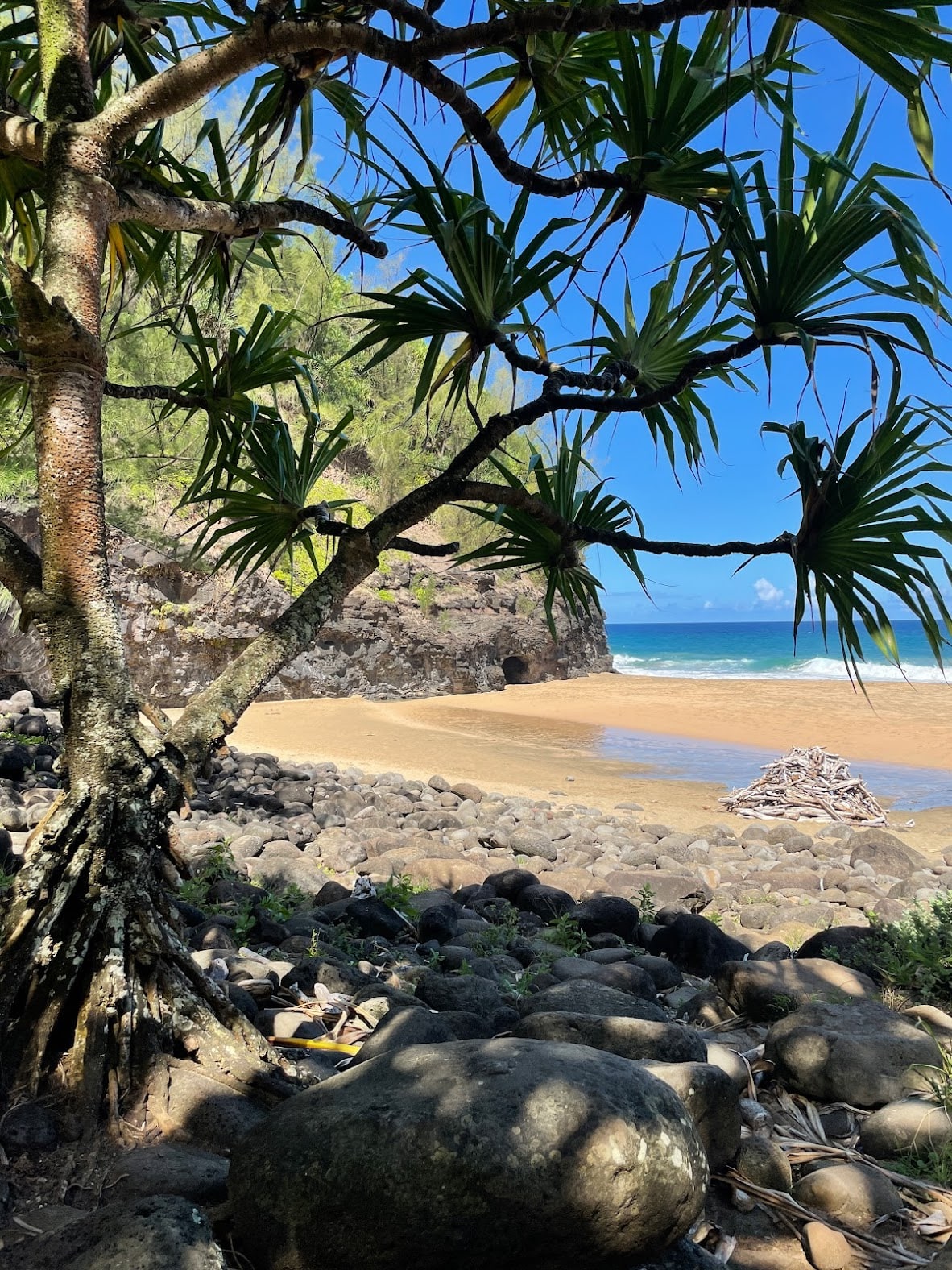
Custom Model Inputs & Outputs
I generated outputs based on a custom input image as well, and also tested transferring the style from new pieces of arts. I used an alpha/beta ratio of 1e-10 because that seemed to be the best middle ground between maintaining the photograph's content and the artwork's style in the generated outputs above.
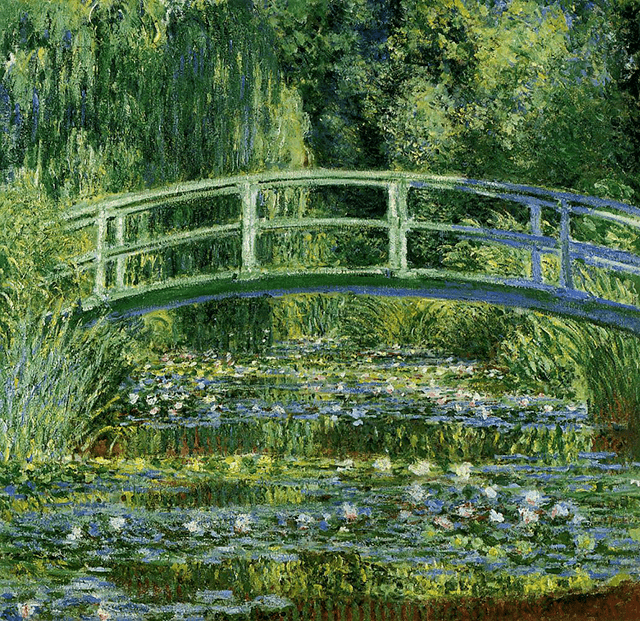
Hanakapiai Beach in Kauai, Hawaii x Water Lilies (Monet)
-min.png)
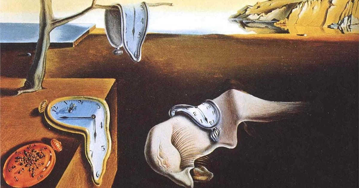
Hanakapiai Beach in Kauai, Hawaii x Persistence of Memory (Dali)
-min.png)
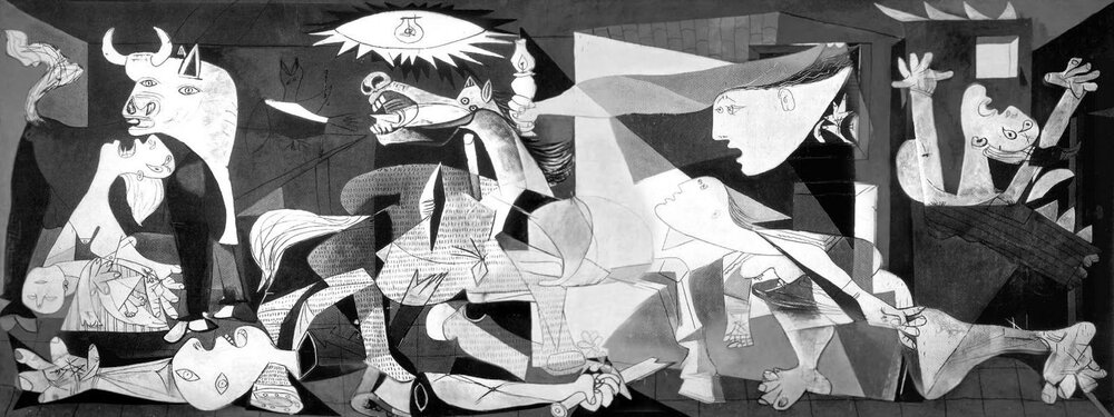
Hanakapiai Beach in Kauai, Hawaii x Guernica (Picasso)
-min.png)

.png)
.png)
.png)
.png)
.png)
.png)