^
Final Projects: Image Quilting, Neural Style Transfer
CS 194-26, UC Berkeley
Yassin Oulad Daoud
Final Project 1: Image Quilting
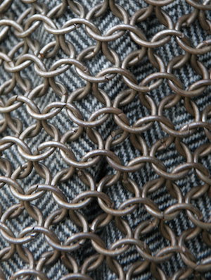
In this first part, I implement the simplest way to perform texture synthesis, which is to randomly sample patches to form an image quilt. I initialize an output image, and, starting from the upper-left corner, randomly sample patches from the input sample image and place them into the output image.
Here are 2 example quilts generated with this method:
Sample input
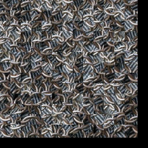
Random quilt
(output size 240x240 with patchsize=20)
The result is not very effective, since the seams between the patches are quite obvious, and the structure of the input texture is lost. Looking only at the random quilt in the above example, it is difficult to tell what the input texture was in the first place.
Sample input
Random quilt
(output size 480x480 with patchsize=60)
In this part, we try to produce a "overlapping quilt" by overlapping our patches and iteratively filling up our output image quilt. We choose the patch with the minimum cost overlap with the previous patch, beginning with a random patch in the top left corner of our output quilt, and adding more patches to the right and down.
To find the minimum cost patch for each iteration, I implemented a helper function get_cost_im which produces a cost image, each pixel of which is equal to the SSD of the overlap between the previous patch(es, if there is both a horizontal and vertical overlap) and the patch from the sample image starting at that pixel. Following the SIGGRAPH '01 paper, I set my overlap width to 1/6 of the patch size. I then implemented a helper function choose_sample which selects the best patch to use by finding the patch with the minimum cost overlap minc (min pixel of the cost image) and randomly choosing a patch whose cost is within a certain percentage tol from that minimum:
y, x = np.where(cost_im < minc*(1.0+tol))
I then place the patch starting at the x, y obtained above with get_cost_im and choose_sample into the output quilt image (overlapping with the previous patches), and repeat until the output quilt has been filled.
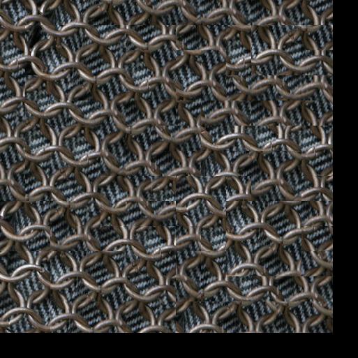
The result is much more effective than the random quilt, since overlapping the patches with the next patch and minimzing the SSD of the overlapping areas make the seams more to notice. Here is an example of an image quilt generated with this method:
Sample input
Random quilt
Overlapping quilt
(output size 240x240 with patchsize=20)
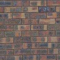
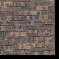
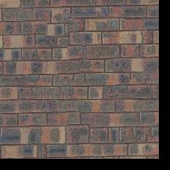
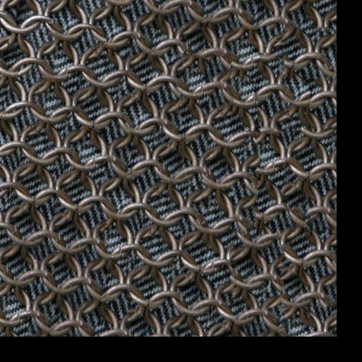
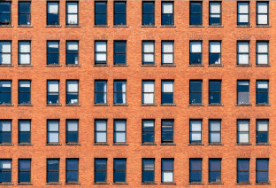
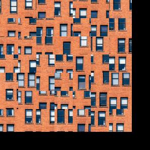
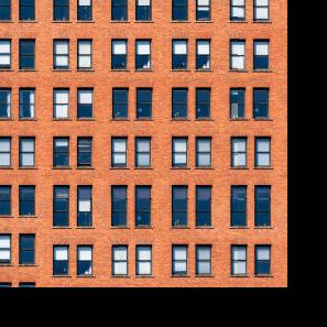
The overlapping quilt still looks a bit flawed, since some of the key structure is still lost (e.g. in the following a brick wall example, the overlapping quilt has some discontinuities in the mortar between the bricks). But you can already tell what the sample texture was just by looking at the overlapping quilt.
Sample input
Random quilt
Overlapping quilt
(output size 480x480 with patchsize=60)
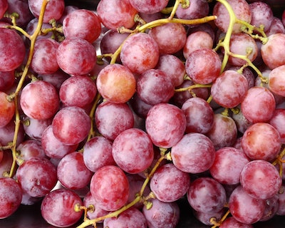
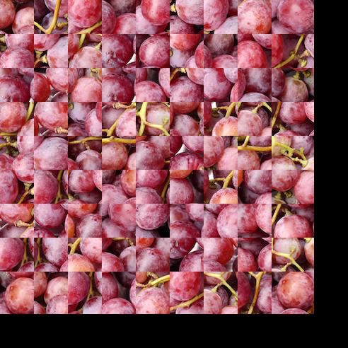
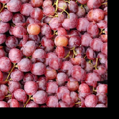
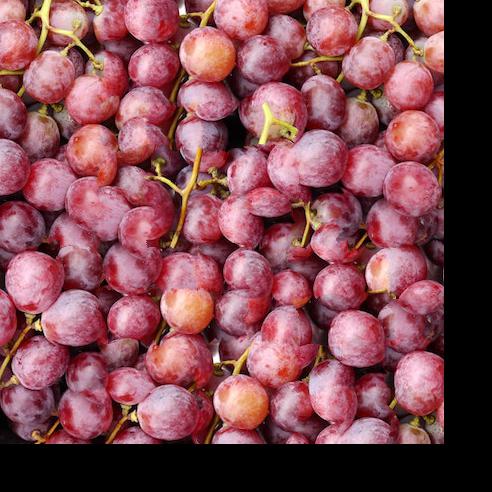
For the grapes, I made the patches a lot larger, allowing most of a single grape to fit in a patch, which is why, even from the random quilt image, one can tell that the input texture was grapes. The overlapping quilt method seems to work poorly for the grapes at such a large patch size, with tolerance set to relatively high (0.1). This is partly because the grapes are round, so straight seams would be more obvious than the brick texture, which already had many perpendicular lines. It could also be because the patches are large, reducing the amount of patches that could yield good overlaps.
With the simple overlapping patches quilt method described above, the seams between each patch will still be quite visible, since the patches are overlapped along straight lines (making the seams more noticable to human vision, which is more stimulated by straight lines). This is especially true for round textures, like the grape example above. In this part, I implement an additional the seam finding procedure, which takes an overlapping region, computes the least-squares cost at each pixel, and computes the minimum path across the region using Dijkstra's algorithm.
Because the sample code for seam finding is implemented in MATLAB, I had to wrote my own cut.py script for this part. A more detailed explanation follows:
I first obtain two overlapping patches--one already in the output, the other a new patch to add--from the "Overlapping Patches" method above (implemented as find_patch). The cut method then takes two patches that have a horizontal overlap and the width of the overlap (if cutting across a vertical overlap, I simply transpose the patches when passing them into cut).

Patch 1

Patch 2
I then compute the least-squares cost of the overlap by squaring the difference between the two regions of overlap from each patch. The resulting cost image is the dark middle strip in the image below. I then pass the cost image into a function cut_path which uses Disjkstra's algorithm to find the minimal cut path over the cost image. The path as a list of pixels is returned, plotted below in red.
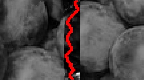
Patch 1 and 2 overlapped, with cost of overlapping region in the middle and cut path.
Lastly, a mask is generated by setting all pixels on one side of the path to True, then the mask is applied to the "old" patch to obtain the new edge of that patch, and the new edge is superimposed onto the overlap region of the "new" patch before it is finally added to the output quilt. The result is a smooth transition between the patches, shown below.
Patch 1 and 2 joined at the cut path
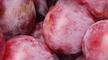
Seam finding greatly improved the quilt generated from the grape input texture. The comparison between the different quilting methods for the grape texture and some others are below:
Sample input
Random
Overlapping
Seam finding
Sample input
Random
Overlapping
Seam finding
Sample input
Random
Overlapping
Seam finding
Sample input
Random
Overlapping
Seam finding

Sample input
Random
Overlapping
Seam finding
Sample input
Random
Overlapping
Seam finding
Sample input
Random
Overlapping
Seam finding
...sometimes randomness is desired!
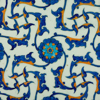
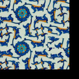
For the texture below taken from one of Boticelli's paintings (guess which!), the texture synthesis as used for the above textures actaully made the generated quilts look too repetitive and unnatural.
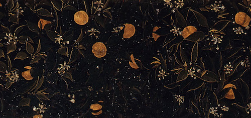
Sample input
Random
Overlapping
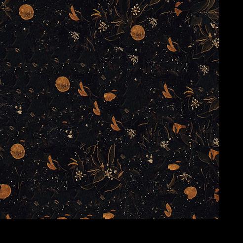
Seam finding
(output size 480x480 with patchsize=60, tol=0.1)
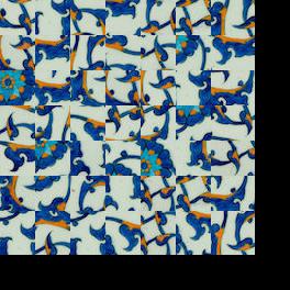
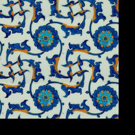
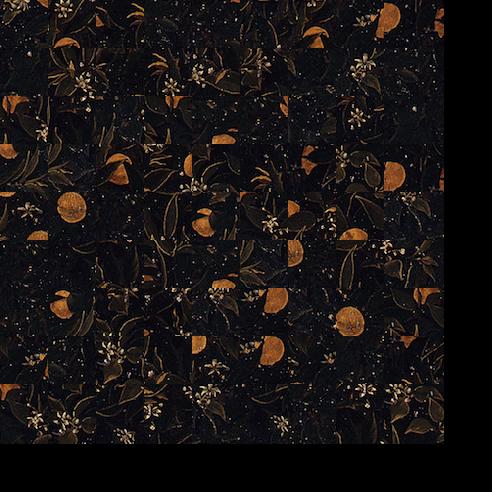
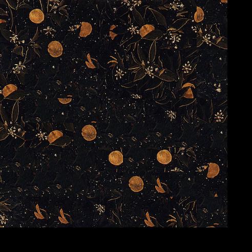
One of the beautiful things about the floral texture here is the natural variation of the forms in the foliage. After generating a quilt with overlapping patches and seam finding, I increased the tolerance by a lot (so that the patches would be chosen almost randomly).
Sample input
Random
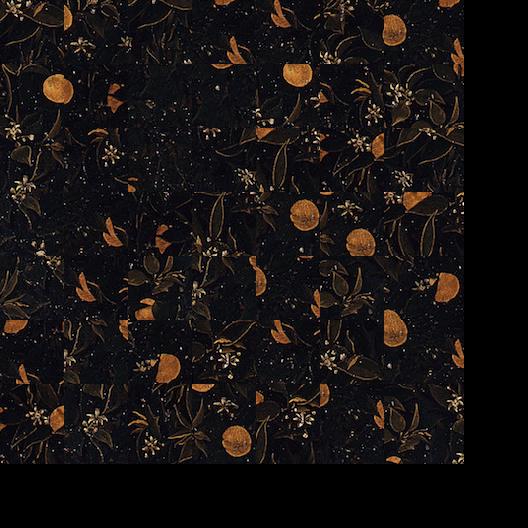
Overlapping
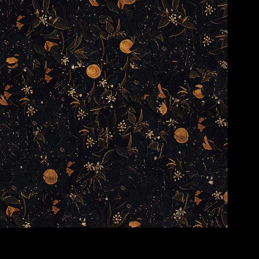
Seam finding
(output size 480x480 with patchsize=60, tol=5)
Increasing the tolerance made the output texture look far more natural; and choosing imperfectly overlapping patches worked since the leaves and flowers already partially cover the oranges in most cases. In fact, even just a using a random selection of patches with seam finding would probably work as well--it's really the seam finding step which gets rid of the unnatural perpendicular cuts that makes the texture look natural.
For texture transfer, we basically want to produce an image quilt that both is both a satisfactory texture synthesis (the methods described above already take care of this) and resembles a target image we provide. When selecting a patch to add to the quilt then, we must include in our cost a measure of how much that patch corresponds to the patch in the same location in the target image.
I mainly just modified the find_patch function I already wrote to take in the target image as an additional parameter. I then modified the get_cost_im function I also already wrote, adding the least-squares difference between the potential patch and the target patch to the cost I already compute for overlapping patches. These two costs are weighted by an alpha value a when added together, so that the total cost for a patch is computed as follows:
cost = a*(overlap cost) + (1 - a)*(target patch correspondence cost)
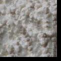
Below is one result from the sample images, with no preprocessing; and the result using the same sample/target images, only this time, a Gaussian filter is applied to the target image before running the texture transfer.
Example 1: input images
Sample image
Target image
Transfer (no blurring)
Transfer (inputs blurred)
Blurring the input images (the sample used for correspondences, and the target image) allows a greater variety of patches from the input sample image to work for a given patch in the target image. This is because the eccentricities (e.g. a flick of the pencil in the above sketch) will be suppressed by the Gaussian blurring before patch selectiong, and yet they will appear later in the generated quilt. This gives the quilt a more "sketchy" and natural look than before.
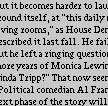
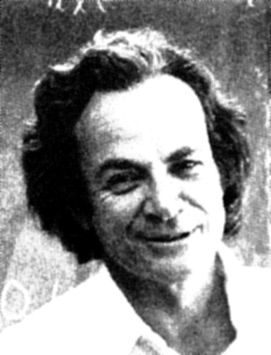
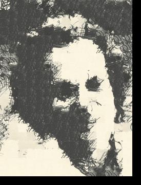
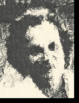
Example 2: Hedgar Allen Poe
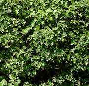
Sample image

Target image
Texture transfer
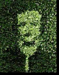
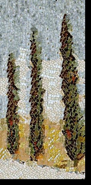
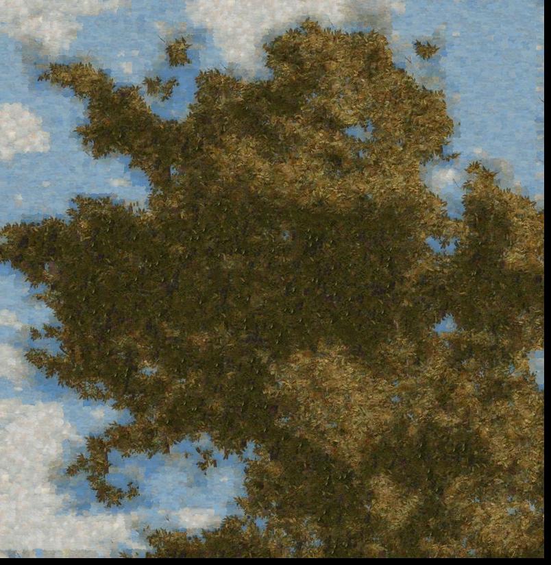
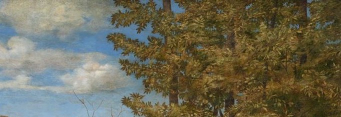
Example 3: Laurel tree from Giovanni Bellini texture
Target image
Texture transfer
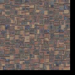
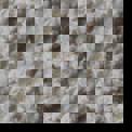
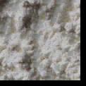
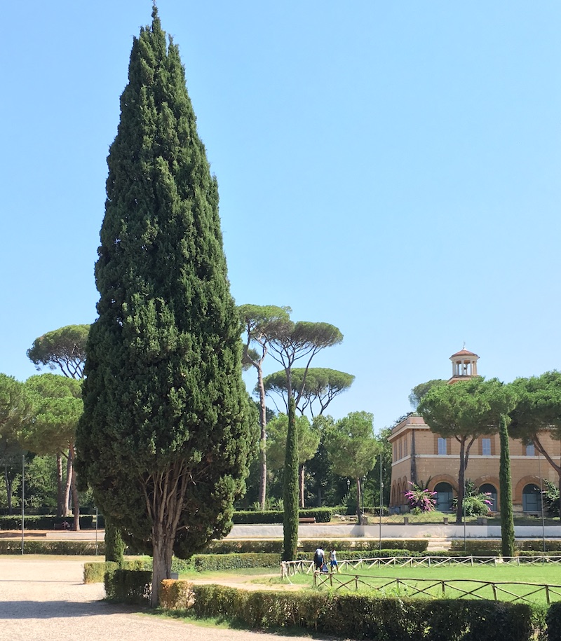
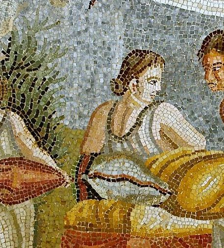
Example 4: Mosaic textures
Target image
Texture transfer
Target image
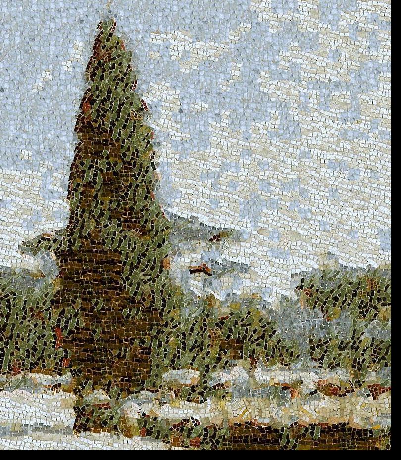
Texture transfer
Special design decisions/issues
One thing I experienced during testing the Texture Transfer part of this project was really slow processing times for certain images (small patch sizes, large images, large overlap values all contribute to longer run time). I noticed that for certain texture transfers with large uniform areas (e.g. a sky or plain background, etc) many patches could work in those areas equally well. To reduce the run time, I added a step parameter which controls the total number of iterations for the patch search over the sample image. Rather than looping over every pixel in the sample image and computing the cost for the patch at that location, the get_cost_im function would now loop over every step pixels. To prevent this new search from being over-deterministic, instead of skipping (step-1) pixels each iteration, I loop over a random sample of (size(image)/step) pixels.
Blending with texture transfer
The above texture transfer technique can render a whole image in a new texture, but what if we want to render the image into an object with a different texture? For this, we would need to somehow "return" the textured transfer image obtained in the previous part to the object from which the texture came.
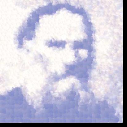
For example, in the "Hedgar Allen Poe" example above, I could make Poe's image look like it is made out of leaves in a hedge, but the resultant image just shows the hedge texture transfer with no context. I will demonstrate how one can make an image seem to appear within another image with the following example, in which I render Leo Tolstoy's portrait in a cloudy scene:
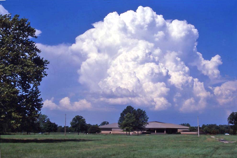
Sample image (OCI)
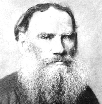
Target image
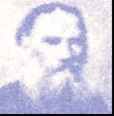
I first perform the texture transfer as in the previous part to obtain an image rendered in a different texture-- the texture transfer image (TTI).

Sample texture
Target image
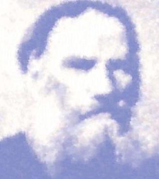
TTI (cropped)
I then superimpose the new image back onto the original image that provided the texture, or original context image (OCI). To deal with artifacts like the edges of the TTI appearing in the OCI, I blend the TTI into a patch of equivalent shape from the OCI, the original context patch (OCP) by using an alpha/beta mask to cross dissolve the images into one another. The alpha mask a is a Gaussian kernel spanning the entire texture transfer image, used to compute the beta mask is b = (1-a). The resulting blended patch is equal to:
blended patch = a*TTI + (1 - a)*OCP
The effect is similar to feathering, by which only the edges of the image are "softened" using a linear alpha dropoff; but by using Gaussian kernel, the feathering is circular about the center of the image, and the alpha dropoff follows a normal distribution, rather than dropping off linearly toward the edges. I vary the extent to which the TTI is dominant by multiplying the Gaussian alpha mask by a given ratio scalar parameter.
TTI
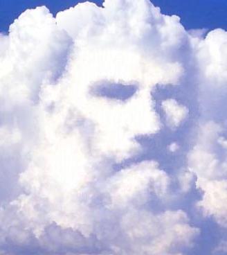
Blended patch
I then add the blended patch back into the OCI at a spot specified by given x- and y-offset values.
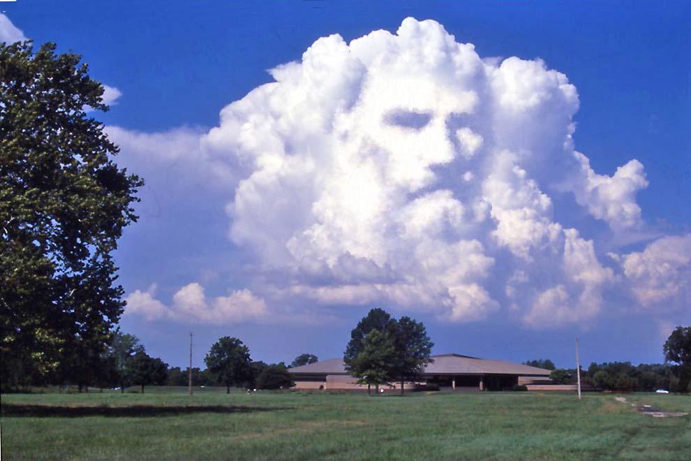
OCI with Blended image
Here are some more examples generated using this method:
"Poest"
Sample/OCI
Target image
Output
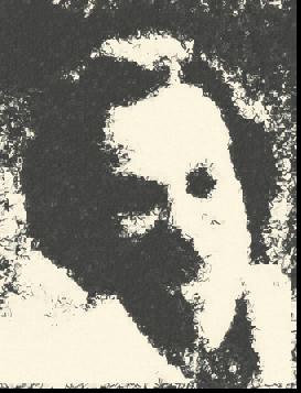
Shakespeare bark
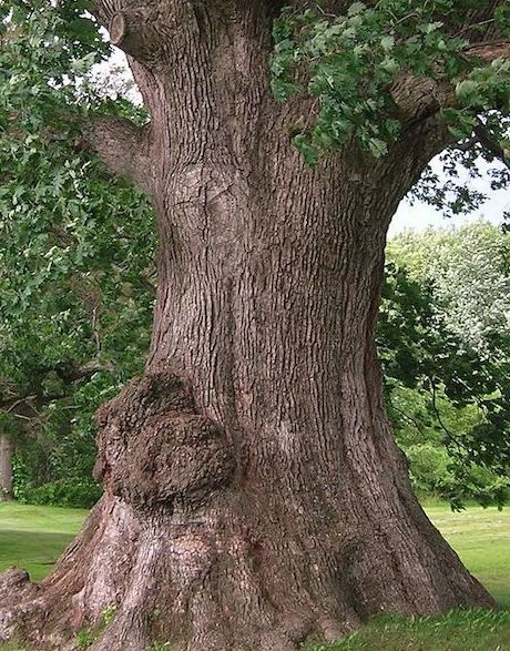
Sample/OCI
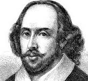
Target image
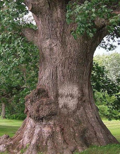
Output
Iterative Texture Transfer
Here I implemented the iterative version of the texture transfer function as described in Efros and Freeman, page 5. The iterative version runs the texture transfer function from before multiple times, in each iteration adding the least-squares difference between a potential patch and what is in the same location in the previous texture transfer output to the existing overlap cost.
I created a separate function iter_texture_transfer which calls the texture_transfer function I wrote before for N iterations. Each iteration i, the patch size is reduced by 1/3, and the alpha value a used to compute the total patch cost during texture transfer is recomputed as:
a = 0.8*(i-1) / (N-1) + 0.1
Below are a couple examples comparing the iterative texture transfer method with the non-iterative one from before:
Target image
Non-iterative
3 iterations
The non-iterative example above captures the form of the target image, but the patches are still somewhat visible. The iterative method on the right above refines the patches in size by the last iteration, capturing more details from the target image and producing better transitions between patches.
Target image
Non-iterative
5 iterations
In this example, it is arguable whether the iterative texture transfer worked better or not. There seem to be fewer/no traces of patches in the iterative version (compare the dark spots in the hair and background between the two); but it looks less "sketchy" since the iterations gradually removed the outlier pencil strokes still visible in the non-iterative version. Where "smoother" texture transfers are desired (e.g. the Tolstoy-cloud example above), the iterative version seems to work better. Where smootheness is not desired, as in this example, it may be best to use the non-iterative version.
Target image
Non-iterative
5 iterations
Python implementation of cut.m
The code provided for the cut function required for Seam Finding is implemented in MATLAB. I wrote a Python version which I used for this project in cut.py. For details on how I implemented the cut, see the Seam finding section above.
Final Project 2: Neural Style Transfer
In this project, I implement the Neural Style Trasfer algorithm by Leon Gatys et al. The algorithm basically uses a pre-trained neural network (I use VGG-19, as described in the paper) to minimize two loss functions, a content loss and a style loss. The content representation is defined as the the match between pixel values from the original image and those in the higher layers in the network, while the style representation is a correlation between filter responses across each layer of the network (Gatys et al. 2).
To compute content loss, I implemented a torch module ContentLoss which simply computes the mean squared error between the input and target images during optimization steps. The method for computing the style loss, as described in the paper, uses a Gram matrix (G_l) for each layer (l) of the network, where each entry (i, j) is the inner product between pairs of feature maps (F) in that layer:
G_l_ij = sum(F_l_i*F_l_j)
The total style loss is then computed as the mean squared error between the Gram matrices from the input and target images (Gatys et al. 10-11). I implemented a torch module for the Gram matrix computation and another for the style loss computation StyleLoss, which computes the Gram matrix for the input image during the optimization and returns the mean squared error between that and the Gram matrix for the target image.
Since the VGG-19 network is pre-computed, it needs to be modified to add the content and style loss layers after certain convolution layers. The paper recommended computing the content loss after "conv4_2" and the style loss after "conv1_1", "conv2_1", "conv3_1", "conv4_1", and "conv5_1." I followed this for my implementation, looping over the layers in the downloaded VGG-19 network and appending the content and style loss layers from the modules described above at the recommended locations (I did not stick with the same naming convention, so my convolution layers are actually "conv_1" ... "conv_16"). Below is the structure of the VGG model I used:
(0): Normalize()
(conv_1): Conv2d(3, 64, kernel_size=(3, 3), stride=(1, 1), padding=(1, 1))
(relu_1): ReLU()
(conv_2): Conv2d(64, 64, kernel_size=(3, 3), stride=(1, 1), padding=(1, 1))
(style_2): StyleLoss()
(relu_2): ReLU()
(pool_2): AvgPool2d(kernel_size=2, stride=2, padding=0)
(conv_3): Conv2d(64, 128, kernel_size=(3, 3), stride=(1, 1), padding=(1, 1))
(relu_3): ReLU()
(conv_4): Conv2d(128, 128, kernel_size=(3, 3), stride=(1, 1), padding=(1, 1))
(style_4): StyleLoss()
(relu_4): ReLU()
(pool_4): AvgPool2d(kernel_size=2, stride=2, padding=0)
(conv_5): Conv2d(128, 256, kernel_size=(3, 3), stride=(1, 1), padding=(1, 1))
(relu_5): ReLU()
(conv_6): Conv2d(256, 256, kernel_size=(3, 3), stride=(1, 1), padding=(1, 1))
(style_6): StyleLoss()
(relu_6): ReLU()
(conv_7): Conv2d(256, 256, kernel_size=(3, 3), stride=(1, 1), padding=(1, 1))
(relu_7): ReLU()
(conv_8): Conv2d(256, 256, kernel_size=(3, 3), stride=(1, 1), padding=(1, 1))
(relu_8): ReLU()
(pool_8): AvgPool2d(kernel_size=2, stride=2, padding=0)
(conv_9): Conv2d(256, 512, kernel_size=(3, 3), stride=(1, 1), padding=(1, 1))
(relu_9): ReLU()
(conv_10): Conv2d(512, 512, kernel_size=(3, 3), stride=(1, 1), padding=(1, 1))
(style_10): StyleLoss()
(relu_10): ReLU()
(conv_11): Conv2d(512, 512, kernel_size=(3, 3), stride=(1, 1), padding=(1, 1))
(content_11): ContentLoss()
(relu_11): ReLU()
(conv_12): Conv2d(512, 512, kernel_size=(3, 3), stride=(1, 1), padding=(1, 1))
(relu_12): ReLU()
(pool_12): AvgPool2d(kernel_size=2, stride=2, padding=0)
(conv_13): Conv2d(512, 512, kernel_size=(3, 3), stride=(1, 1), padding=(1, 1))
(style_13): StyleLoss()
(relu_13): ReLU()
(conv_14): Conv2d(512, 512, kernel_size=(3, 3), stride=(1, 1), padding=(1, 1))
(relu_14): ReLU()
(conv_15): Conv2d(512, 512, kernel_size=(3, 3), stride=(1, 1), padding=(1, 1))
(relu_15): ReLU()
(conv_16): Conv2d(512, 512, kernel_size=(3, 3), stride=(1, 1), padding=(1, 1))
(relu_16): ReLU()
(pool_16): AvgPool2d(kernel_size=2, stride=2, padding=0)
I normalize the inputs using a fixed mean and standard deviation as recommended in this post. I also changed the max pooling layers to average pooling as suggested on page 9 of the paper.
The loss from the content layer and 5 style layers are combined in a weighted sum and backpropogated during the optimization loop. As shown in Figure 3 of the paper, the style weights should generally be a lot larger than the content weight and should generally decrease from the first to the fifth content loss layer. I had to play around with the weights I used, since varying them for each image seemed to produce the best results; but I set the default style weights to [style1=100000, 10000, 1000, 100, style5=50] and the default content weight value to 1, matching the descending ratios shown in Fig. 3 of the paper.
Same image from Gatys et al. combined with various paintings
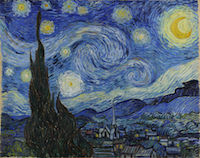
Van Gogh
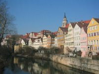
Tübingen (from paper)
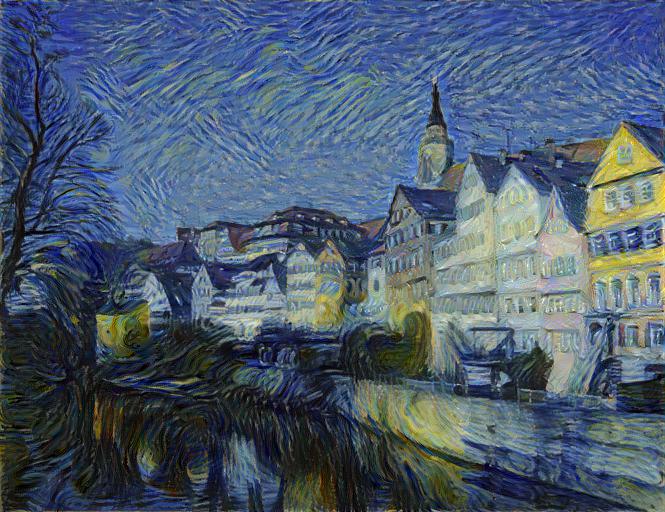
Style transfer (my result)
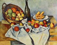
Cezanne
Tübingen (from paper)
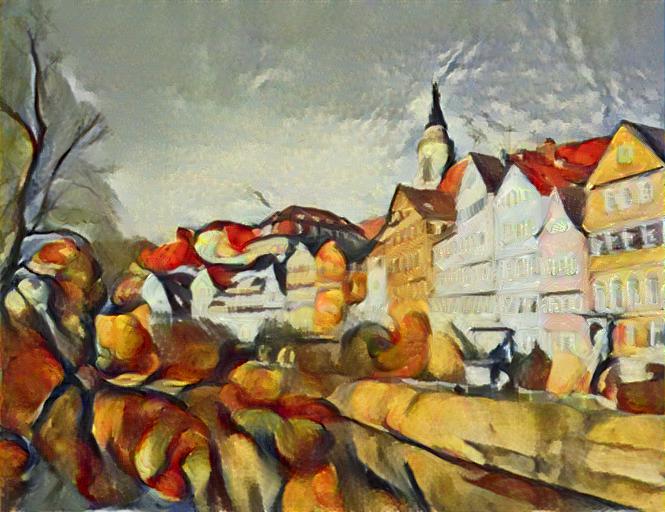
Style transfer
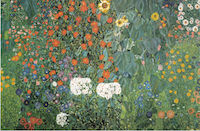
Klimt
Tübingen (from paper)
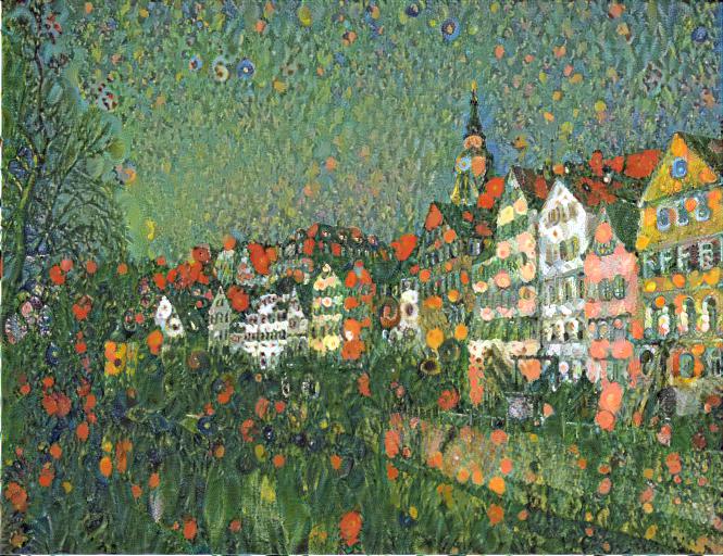
Style transfer
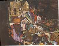
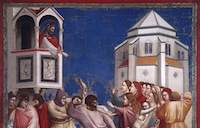
Schiele
Tübingen (from paper)
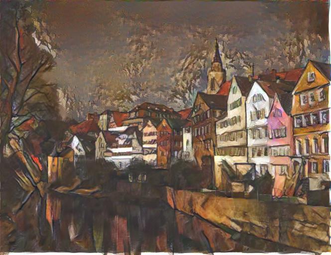
Style transfer
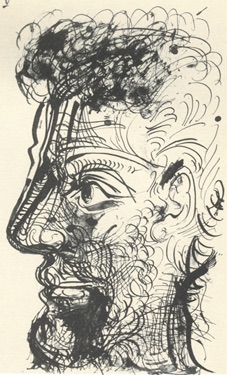
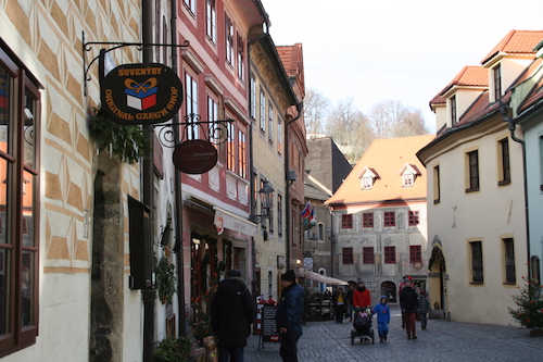
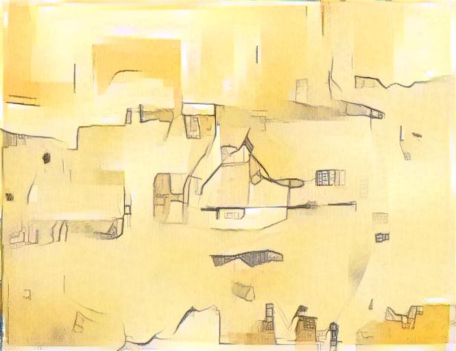
Egon Schiele and images I took at Česky Krumlov
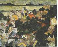
I was looking through Schiele images to use for samples, and found this sketch:
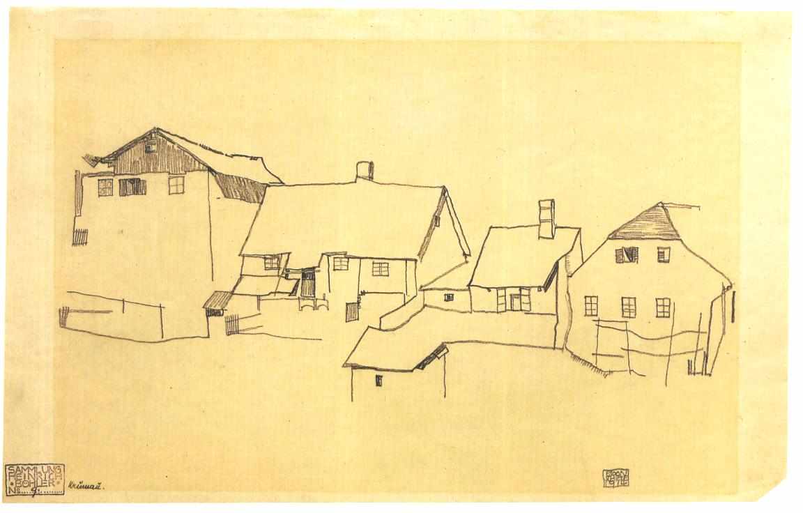
It seemed so familiar, and it struck me that it looked like this row of houses in the Czech Republic I had seen when I went to that same town some years ago! I even made my own painting of this same row of houses! I found the photos I had taken there on my trip and decided to make a few Schiele versions of them using the methods I learned in this project:
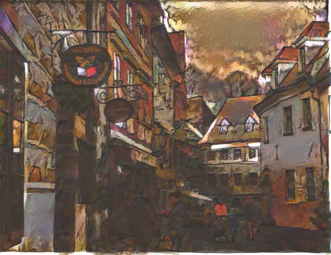
Schiele
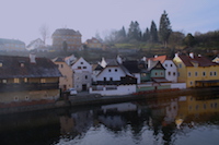
Česky Krumlov (my photo)
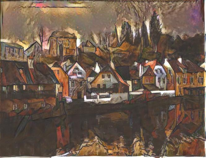
Style transfer
Schiele
Česky Krumlov (my photo)
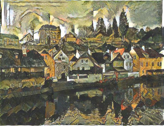
Style transfer
Schiele
Česky Krumlov (my photo)

Style transfer
Schiele
Česky Krumlov (my photo)
Style transfer
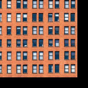
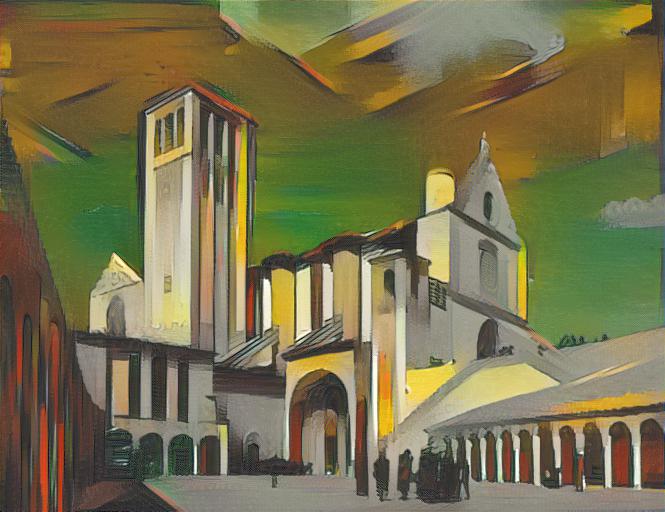
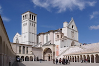
Medieval/modern? Giotto and Giorgio Di Chirico
One of the moments I had been waiting for this whole course was to implement this project so I could finally make my own Giottesque versions of Italian Gothic buildings, and the Basilica of Assisi has to be my favorite. There is such a surreal quality to the architecture from this time and place (probably the simple, massive shapes and romanesque arches) that reminds me of the Italian surrealist Giorgio de Chirico and his sublime cityscapes:
Giotto
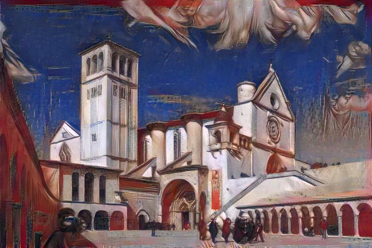
Style transfer
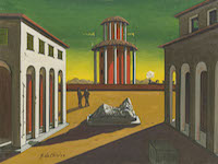
De Chirico
Style transfer
Klimt and the Huntington Library rose gardens in Pasadena, CA
Klimt
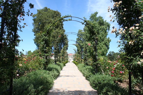
Huntington gardens (my photo)
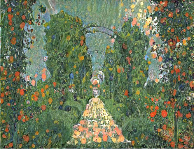
Style transfer
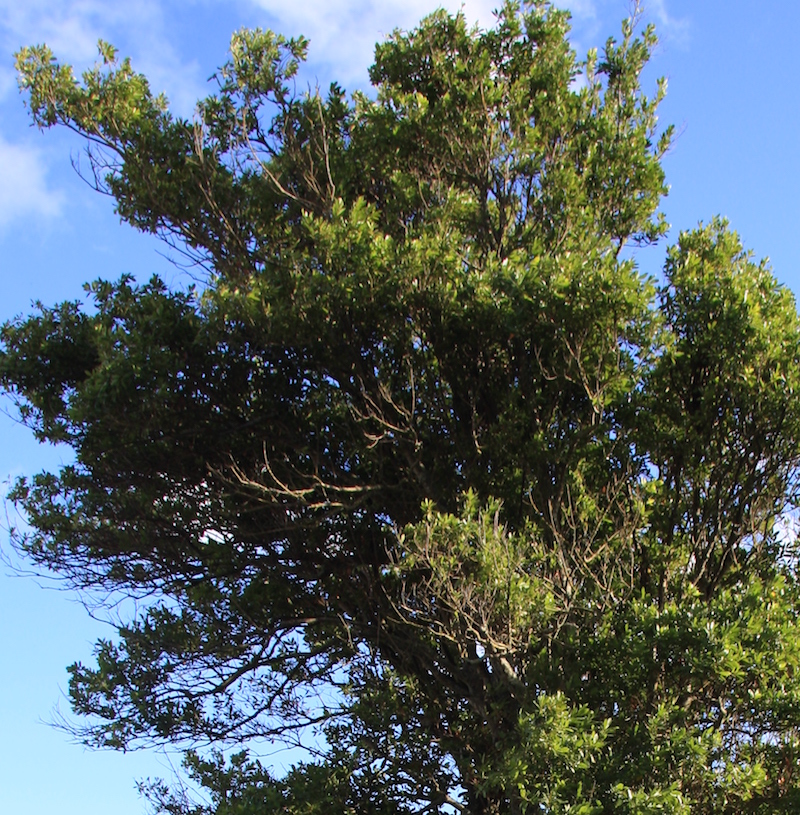
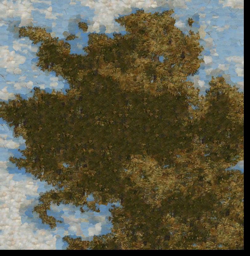
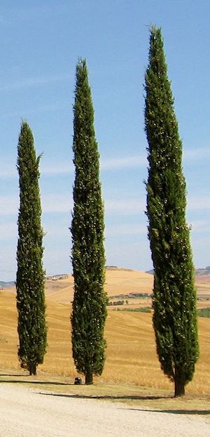
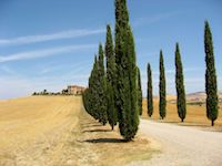
Van Gogh cypresses in Tuscany
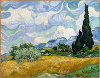
Van Gogh
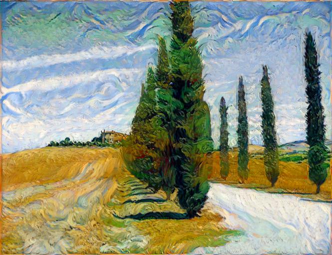
Style transfer
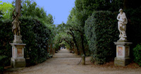
Boboli Gardens as Boticelli
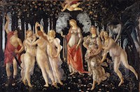
Boticelli
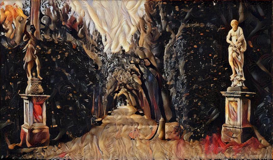
Style transfer
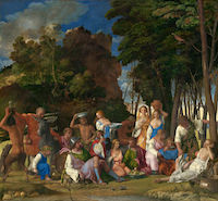
Bellini
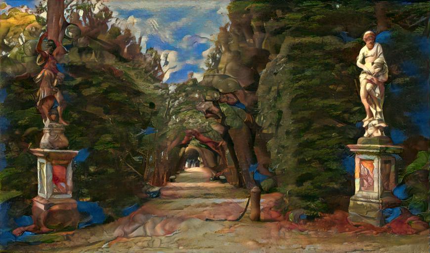
Style transfer
This style transfer actually worked pretty well, in the sense that the content of the original image was captured pretty accurately (e.g. the groun, foliage, sky, etc. are not mixed up too much). It just doesn't feel like Bellini's style was captured very well, and this might be because the Neural Style Transfer method works less successfully with paintings that have high enough naturalism/ more subtle stylistic distinction. The Boticelli transfer from the same gardens image above looks a bit stranger (e.g. the sky is made up of the nymphs' robes); but I get the sense of Boticelli more from that image, probably thanks to all the eccentricities left in the style transfer.
Schiele
Česky Krumlov (my photo)
Style transfer
Unfortunately, the sketch by Schiele that suddenly meant so much to me did not work that well for the style transfer, even though some of the buildings are present in both the input and target images! The resulting image does look quite interesting all the same.
Image Quilting
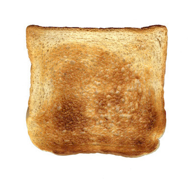
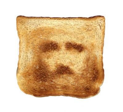
I really enjoyed that the results of this project felt "smart"--as if the project involved machine learning techniques to "learn" textures and transfer them--but it didn't! The was honestly surprised that image quilting algorithm worked so well, especially after the "Seam Finding" step was implemented. While doing the texture transfer portion and the Bells and Whistles for the project, I also learned that being selective about examples and choosing sample images that intuitively would seem to work well as quilts is extremely important for achieving good results (e.g. "faces in toast" works as a texture transfer, but "faces in blank sheets of paper" won't).
Neural Style Transfer
The reason I did these two projects for my final was because they seemed to address related problems of "transfering" (or extending) qualities of one image onto another. Unlike the first project, this second project did involve machine learning, so I was able to get a sense of how this general problem in computational photography works from a non-deep learning and a deep-learning perspective. For this reason, the Neural Style Transfer project was a bit more challenging to re-implement, since the margin between "good" and "bad" results is finer and yet more obvious--I spent a lot of time just trying to get my implementation to produce a single decent style transfer. I was worried my results would not be good since I had seen the project webpages of previous semesters of this course, and many students did not seem to achieve good results. I was surprised by some of the results I managed to get, since in some cases they were better even than those from Gatys et. al (e.g. compare the Van Gogh/Starry Night transfer shown in the two). I learned more about which kinds of sample pitcures work better (heavily and systematically "stylistic" images, e.g. Impressionists, other modernists) and those which do not work as well (Early Modern European paintings, and other "naturalistic"/subtly stylistic traditions). Achieving good results, again, came down to keeping this in mind and choosing input images that would work together (maybe they share one striking feature--a tree or houses, etc. that would immediately capture the input artist's "hand").
These projects taught me a lot about how digital images share qualities and can be extended beyond just their original state to produce new and interesting images. It forced me to think about the artworks as well, and this unanswered question of style in the arts, on which computation seems to be able to shed a bit of light. This was probably my favorite CS class I've taken so far, and I'm really grateful for everything I've learned through these amazing projects!