In the least-squares setup, A is a matrix that has one row for every pixel in
S that admits an x gradient (i.e. not the last pixel in its row), one additional row for every pixel that
admits a y gradient (i.e. not the last pixel in its column), and one row for the corner constraint.
Each x-gradient row of A has two entries: a -1 which is multiplied by v(x,y) and a 1 for v(x+1,y).
The vector b contains the corresponding value of s(x+1,y) - s(x,y). The process is analagous for y-gradients.
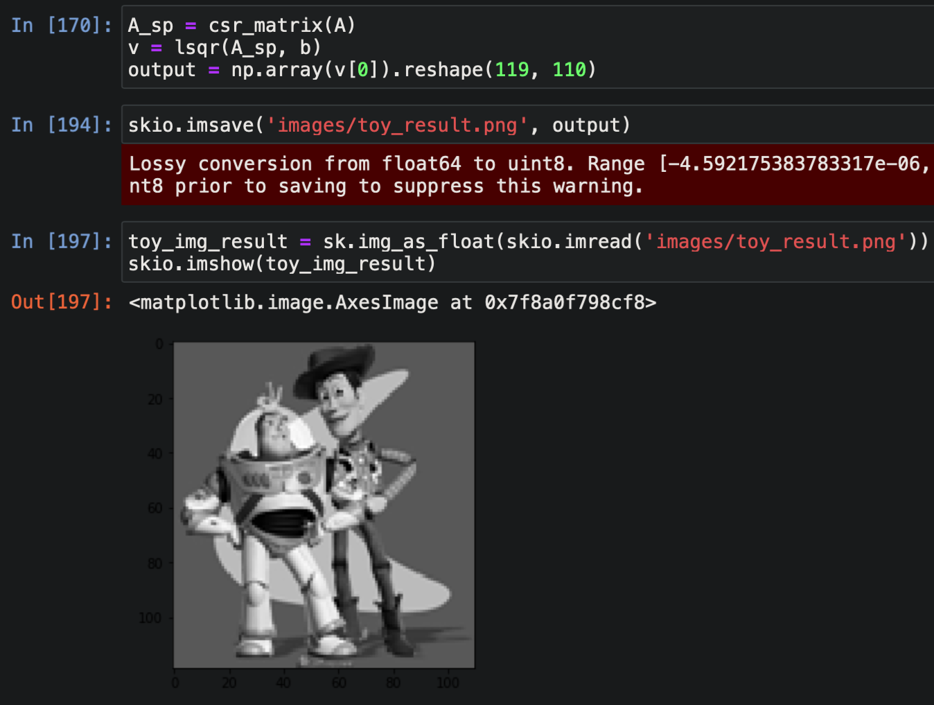
To turn the pixels in S into a solvable vector v, we map each (x, y) pair to a pixel ID in [0, ..., |S| - 1].
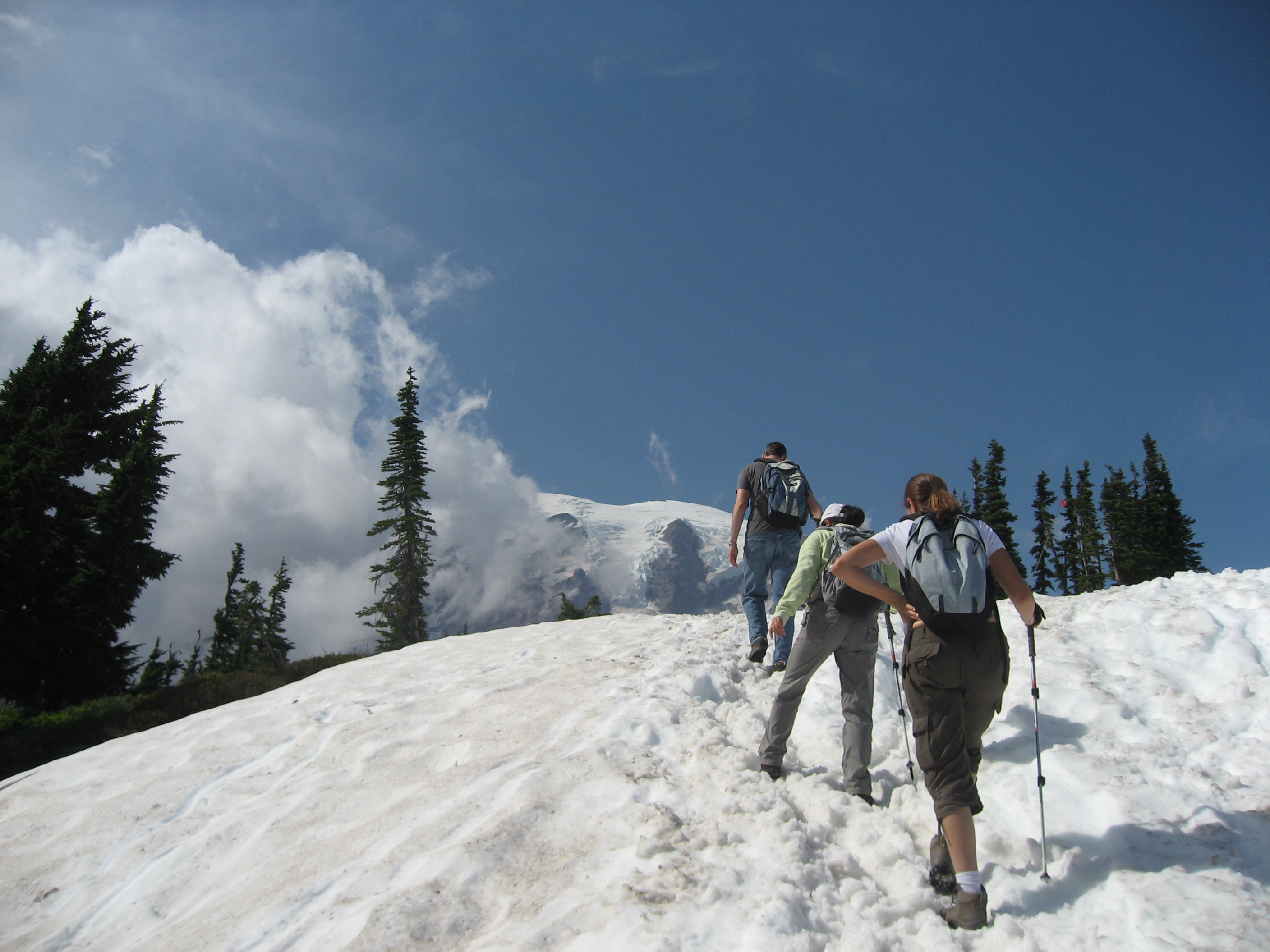
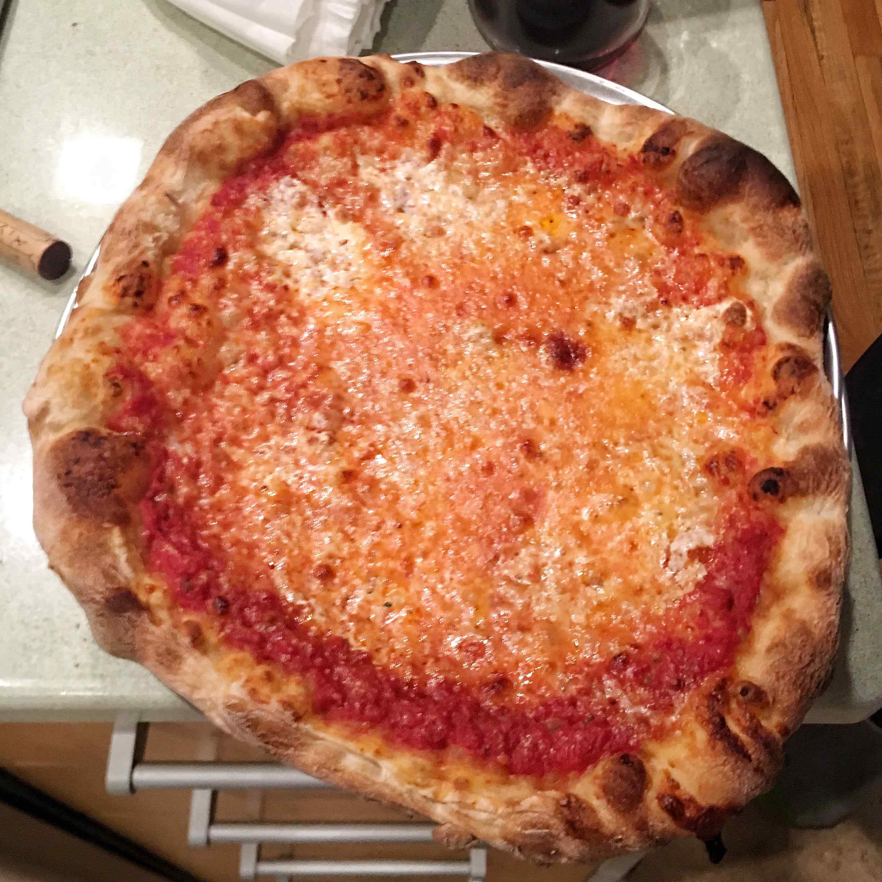
The results match the original image:

For Poisson blending, I modified the approach above to include the boundary (t_j) losses in the least-squares setup. To do this, we add additional rows to A for each boundary pixel in S, as well as an additional entries in b equal to the appropriate s_i - s_j + t_j from the second summation above.

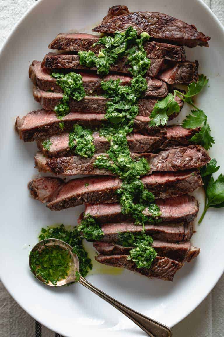
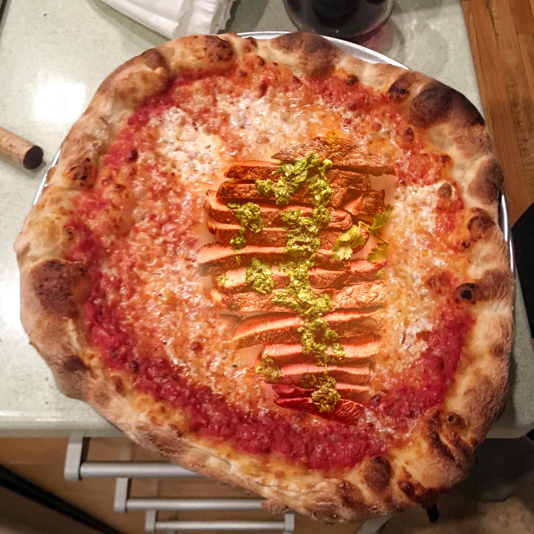
The last image doesn't turn out as well because the white background of the steak is a significantly different color than the orange and red of the pizza.
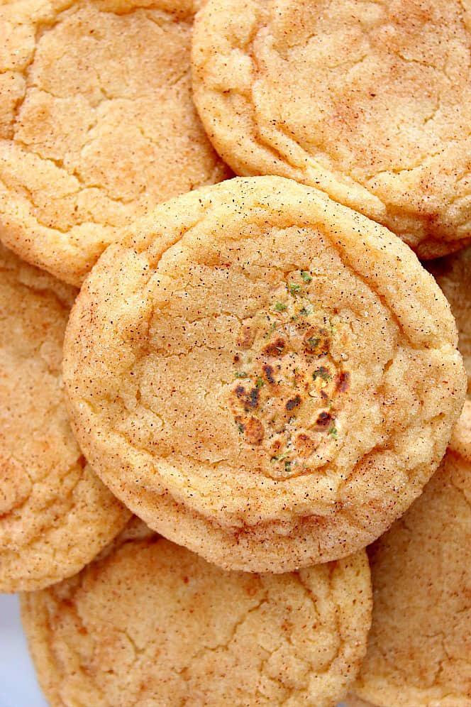
The mixed gradient approach is much better at incorporating information from the target
image into our blend due to its inclusion of target gradients; this produces better
results when the texture of the target image within the source region is something we
want to preserve.
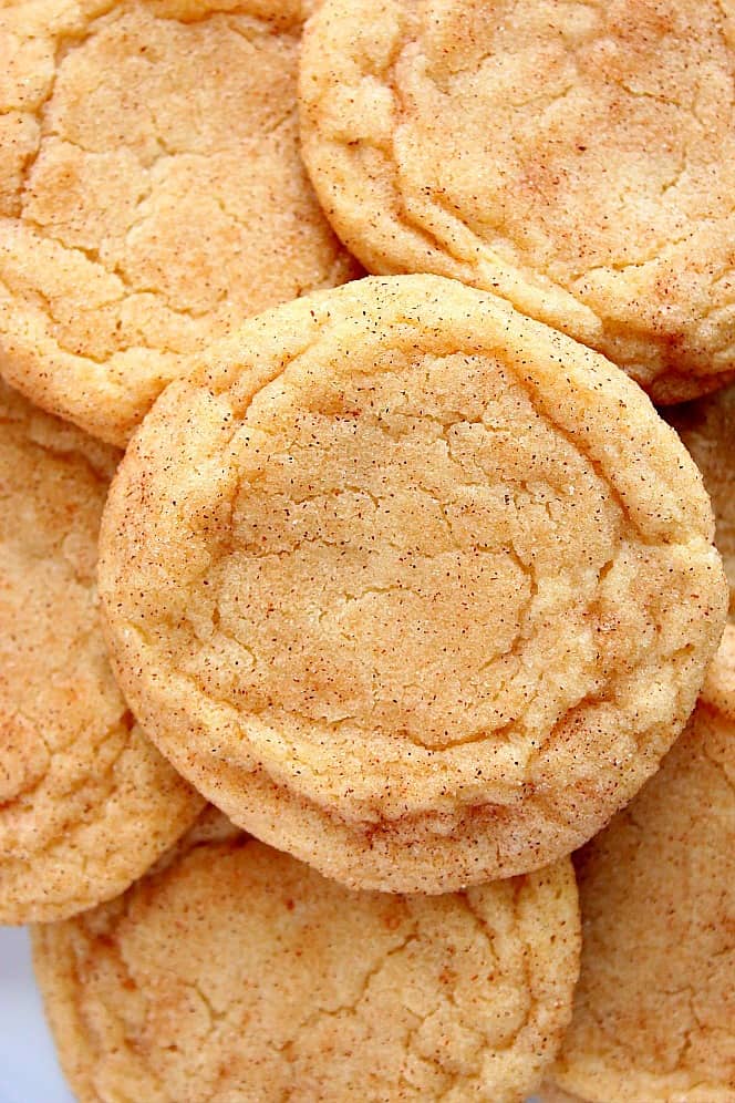
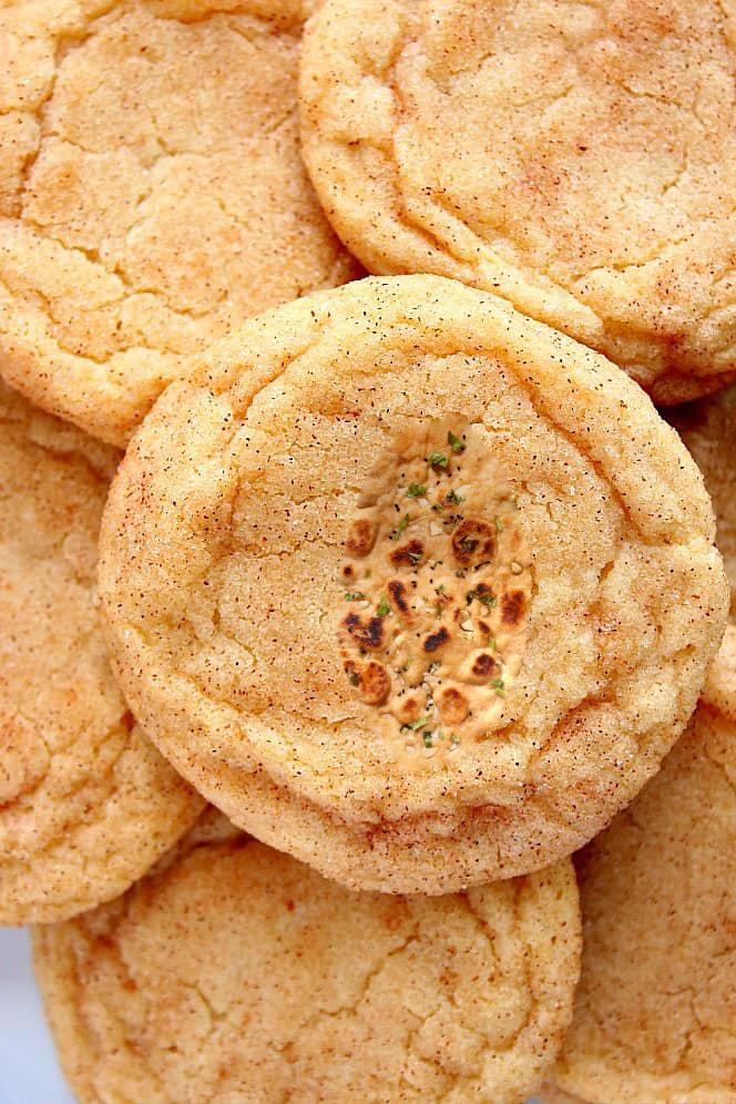
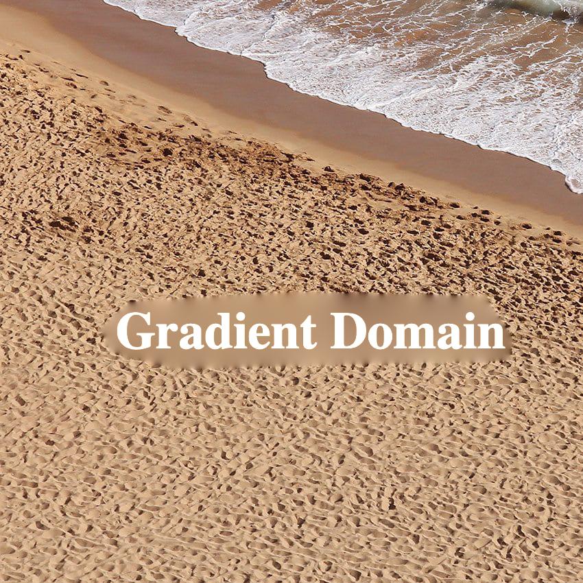
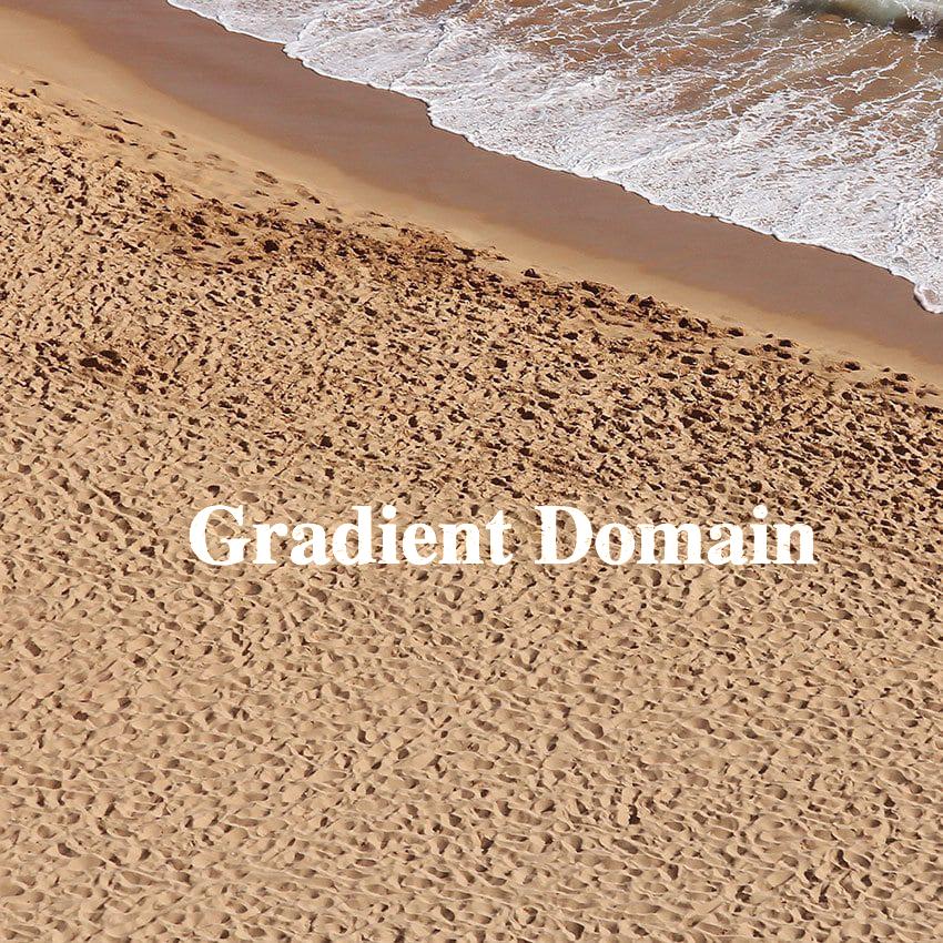
For example, the grooves of the sand and the small black dots of the cookie are much more
visible within the blended region after we switch to mixed gradient. Additionally, the
transition from bread to cookie is noticeably more seamless.
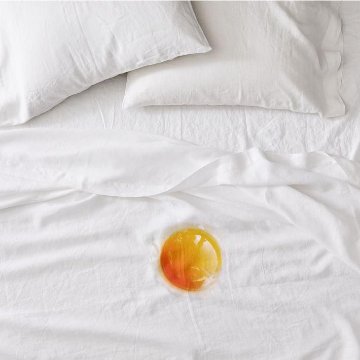
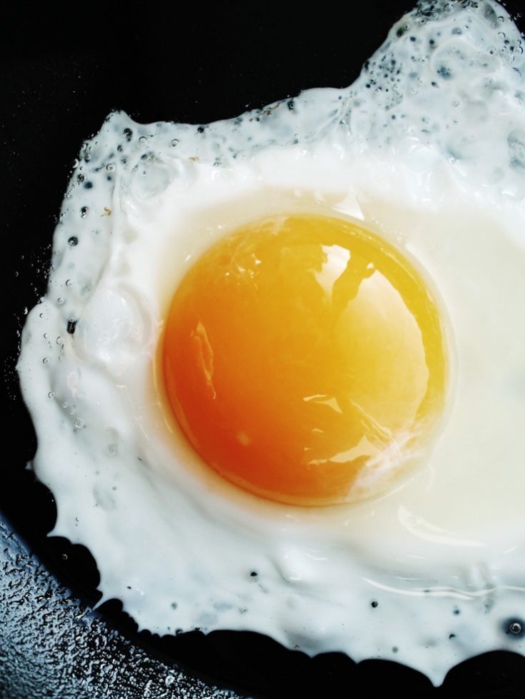
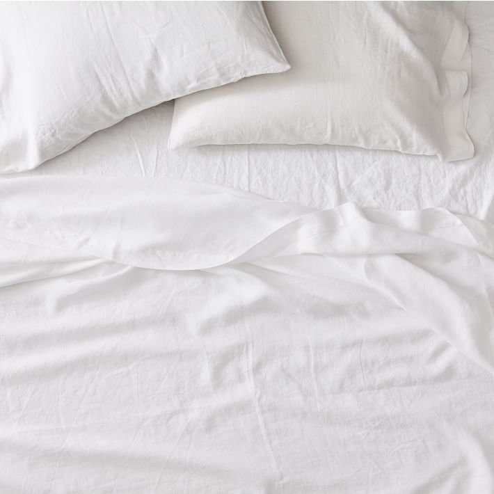
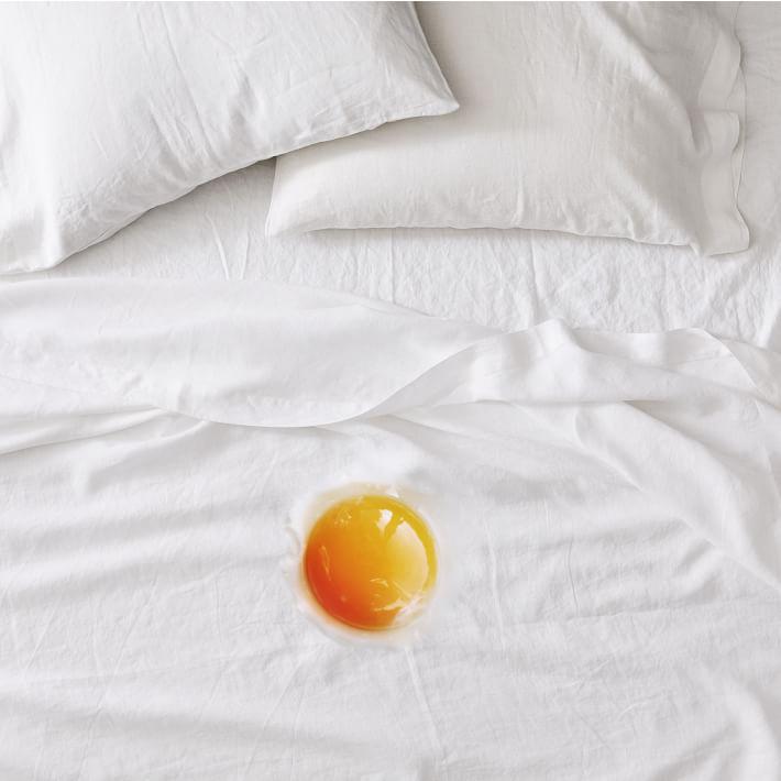
This effect is not always desirable. In this last case, using mixed gradients displays some of the wrinkles in the bedsheets through the yolk of the egg, so our original method is better.
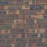
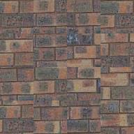
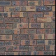
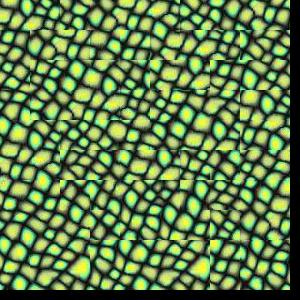
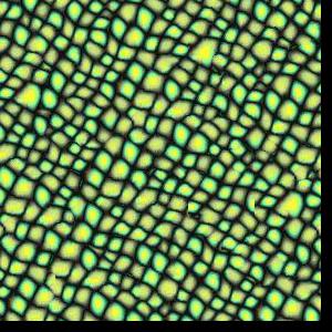
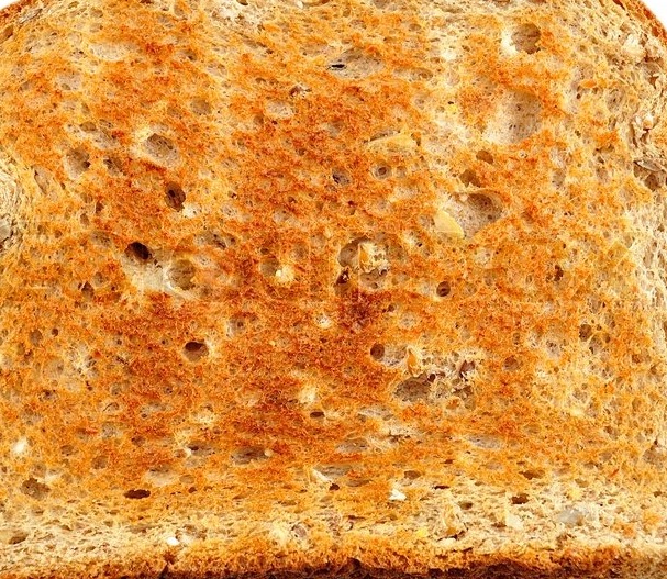
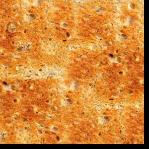
Using this approach, we can still see pretty clearly the borders between different patches in the right image. The patch size here is 48 (1/4 of image length/width).
To implement overlapping patches, I started with the suggested helper functions, and used convolution when computing the SSD.
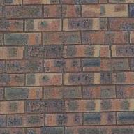
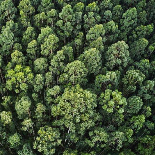
In this example, we sample the lowest-cost patch based on the values in the SSD image, after setting the top left patch of the result image to be that of source image. As expected, we get a copy of the original image. Here the patch size is 40 and overlap is 10.
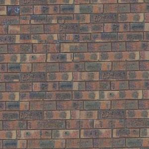
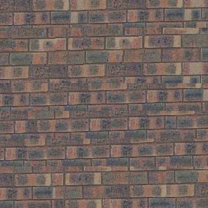
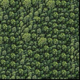
In this approach, we sample one of the K lowest-cost patches based on the values in the SSD image, and select the top left patch of the result image randomly. Here the patch size is 48, overlap is 24, and K is 2. The results are better than the completely random sampling above, but seams are still visible.
Instead of using the given code, I implemented min-cutting from scratch using dynamic programming, as suggested.
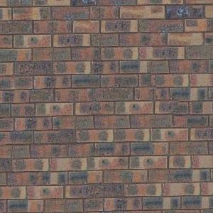
The seam finding approach significantly outperforms the previous simple overlapping approach, with less visible seam artifacts present.
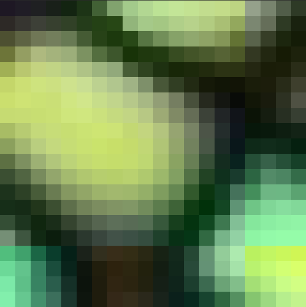
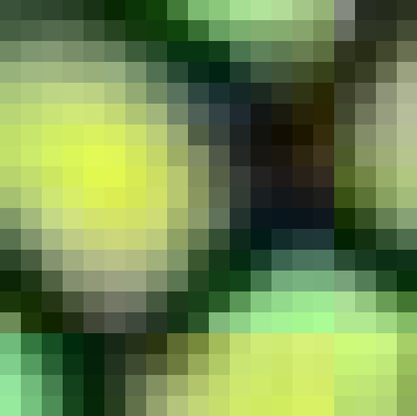
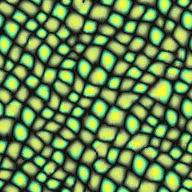
Above is an example of overlapping regions used during generation of the first seam finding example. As we can see, the regions are relatively similar toward their top half, but become quite different at the bottom. As such, we probably want the cut to run across the upper section to make the transition as seamless as possible.
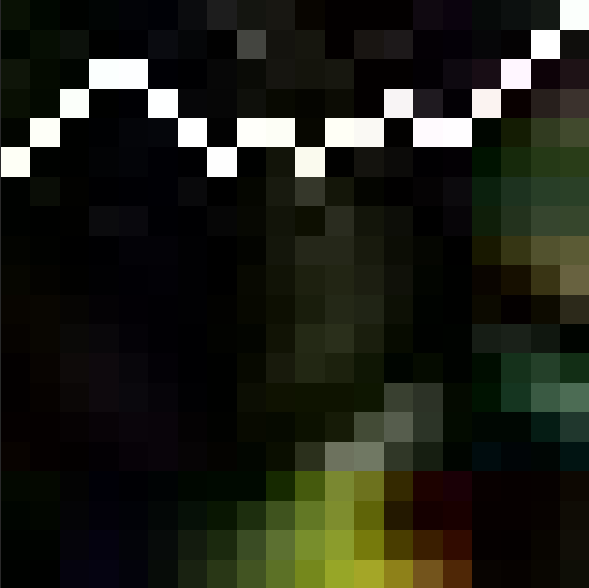
As expected, the path (in white) runs through the upper part of the regions.
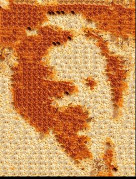
To implement texture transfer, I simply modified the SSD image used in the past two approaches to assign a cost to each possible sampled patch, adding to it the SSD between the original "shape" image we are trying to recreate and the texture image.