Part 1: Depth Refocusing
Finite Difference Operator
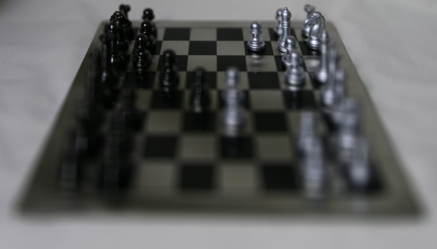
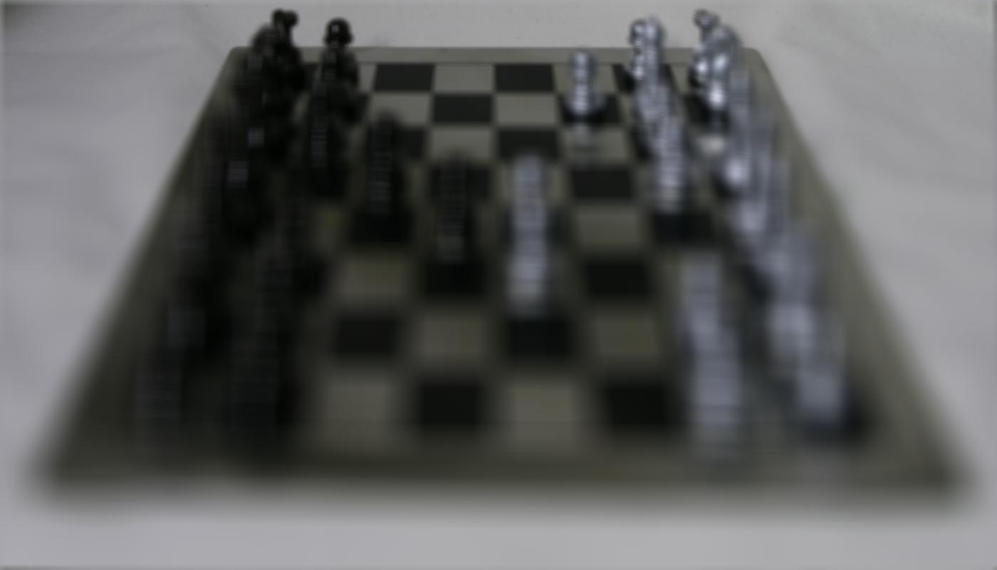
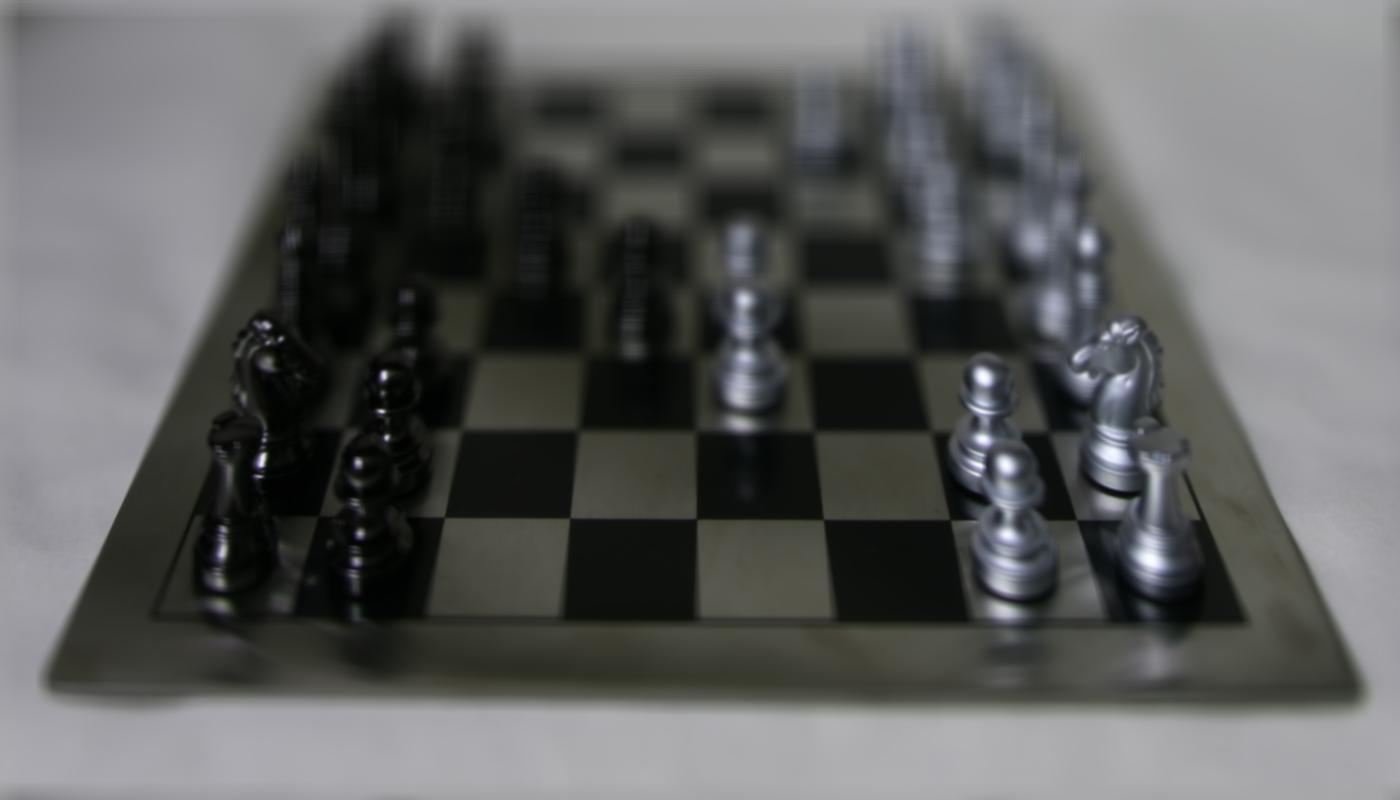
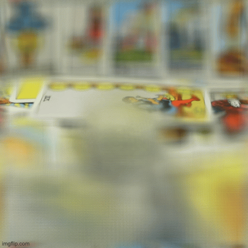
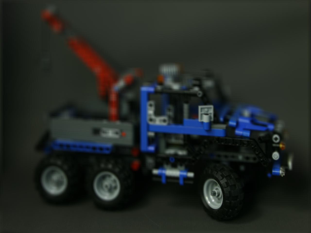
To refocus the image, I iterated through the grid of images and shifted all of them towards the middle image, which was found at (8, 8), since the cameras were in a 17x17 grid. The file names provide us with the absolute positions of the camera, but to perform the shifts, we have to choose an image to shift towards. Then, we get the image we will be shifting, and its absolute positions. We subtract this from the absolute position of the center view, and scale this by c, which is a parameter we select and adjust to change the point of focus. These calculated shifts are our dx and dy, which we use to np.roll the image by in order to perform the transform. After we perform all of the shifts for each image, we take the average of all of these images, which returns the final view with the depth refocused.
|
|
|

|
|

|

|
|

|
|
Part 2: Aperture Adjustment
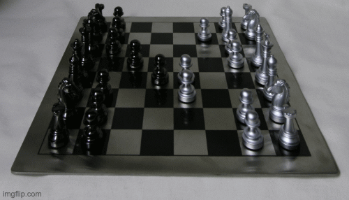
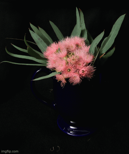
To perform aperture adjustment, we use the shift function from the previous section to generate all of the images at a certain depth (determined by c). However, instead of taking the average of all 289 images, we instead pick a radius of images we want to average. I select the middle square of images of size radius x radius, and these are averaged to create the final image. From the results, we can see that a small radius simulates a small aperture, as there is only one view, similar to a pinhole camera, so everything is in focus. As the radius is increased, the aperture does too, creating a depth of field effect that causes elements not in the focus point to blur. This is the effect of the increasing number of images to average. As the radius becomes 8, we recover the original image from the previous section.

|

|
|

|
|

|
|

|
Summary
It was really cool to use the light field image data to simulate some of these effects. I took Professor Ren’s 184 class last spring, and while we touched on the light field cameras, this project really solidified the ideas he talked about in class. I think initially, I was confused on how to use the image file names as data for the depth refocusing, which made it difficult to start, but once I was able to extract and use that, the project was more fun than complicated. I enjoyed learning about this technology and how it ties to the plenoptic function that we talked about in class. It was pretty cool that we could take advantage of these minute differences in images and turn them into camera effects that are usually implemented by the hardware of a camera.