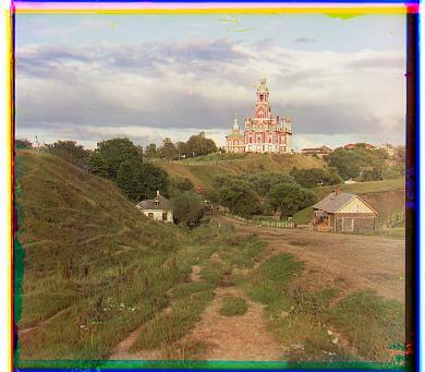
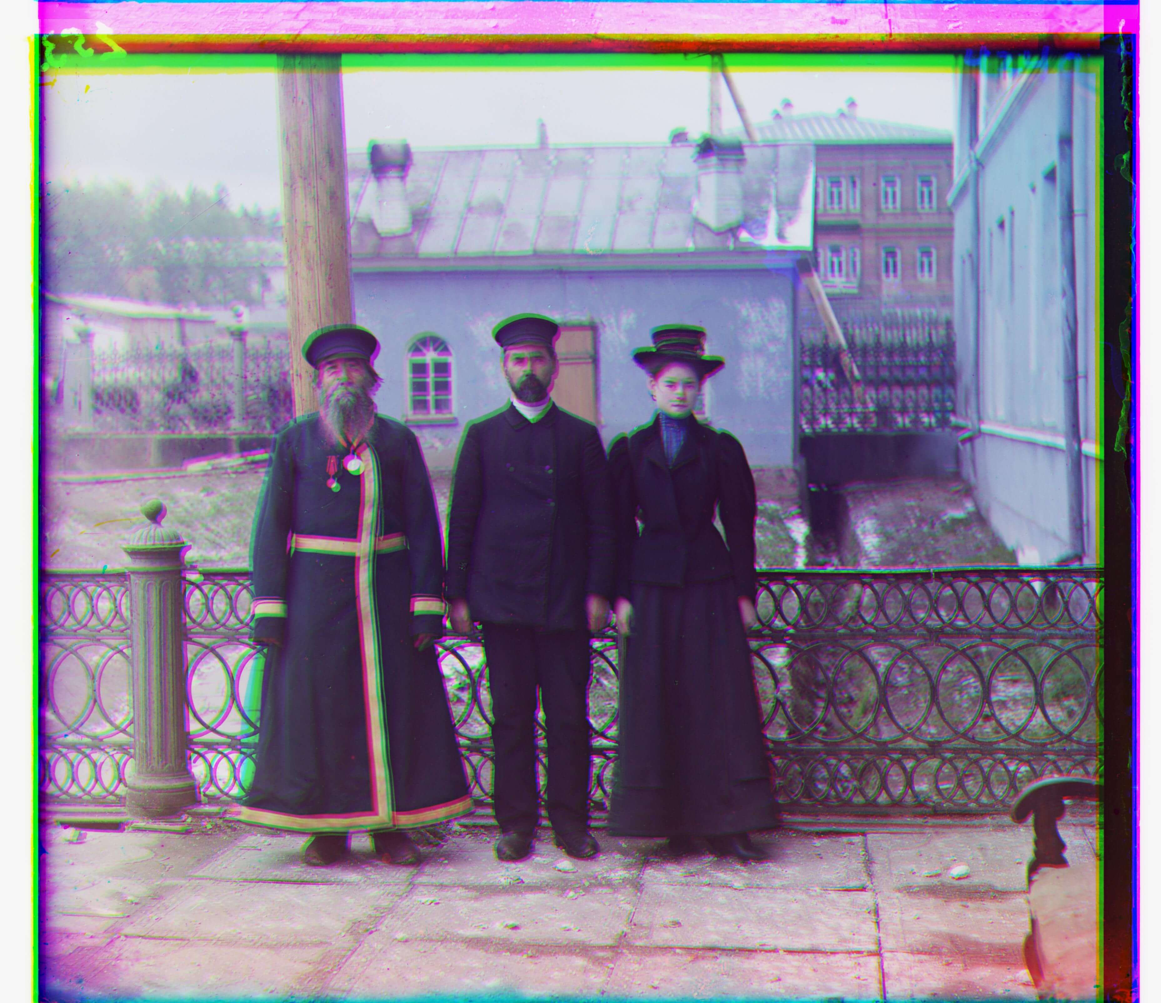
cathedral.jpg
G: [2, 5]
R: [3, 12]
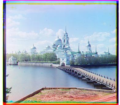
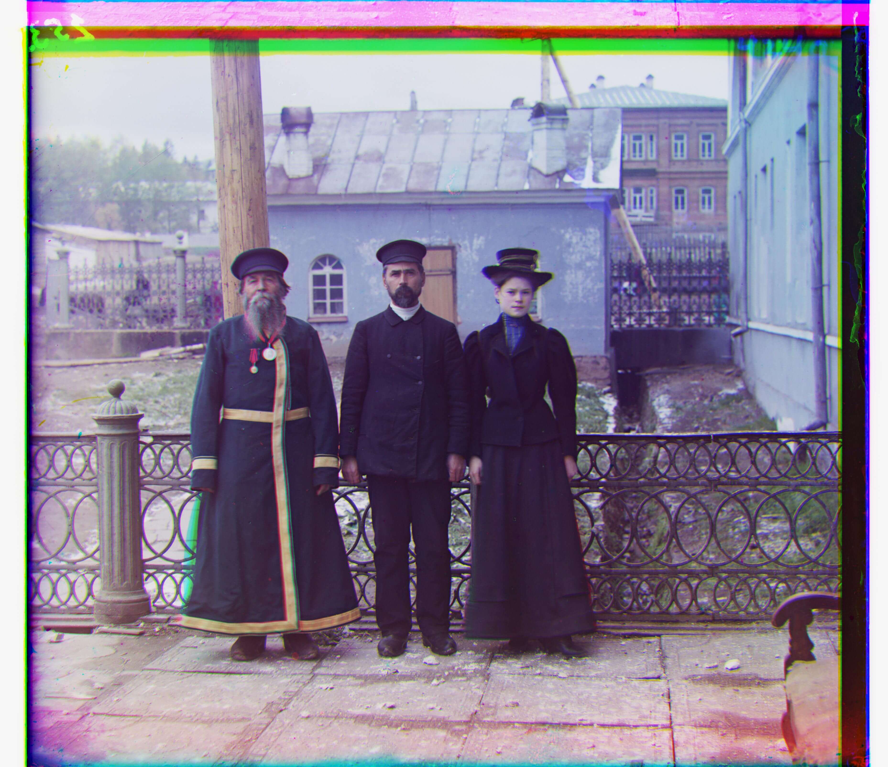
monastery.jpg
G: [2, -3]
R: [2, 3]
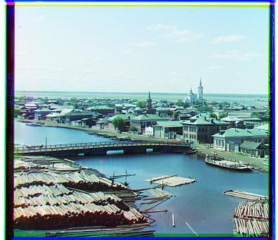
tobolsk.jpg
G: [3, 3]
R: [3, 7]
As early as 1907, Sergei Mikhailovich Prokudin-Gorskii, a Russian chemist and photographer,
traveled across the vast Russian Empire and took color photographs of everything he saw. He
was able to do this by recording three exposures of every scene onto a glass plate using red,
green and blue filters. The three filtered photographs can then be superimposed into one full
color photograph if aligned well. Although he had grand plans to show the colorful world of
Russia to the youth, his plans never materialized and he left Russia, never to return
again.
Fortunately, his RGB glass plate negatives survived and were purchased by the Library of
Congress in 1948. They have recently been digitized, and were the images that I worked with
for this project. The main goal of this project was to create a program that took the RGB
filtered images and aligned them correctly, within an average running time of less than 1
minute.
Before we begin the main process of aligning the RGB filtered images, we must preprocess what we are given: an image showing a vertical stack of the filtered images (given as a matrix). Specifically, from top to bottom, there is blue, green and then red. Therefore, all we need to do is divide the given image into thirds (from top to bottom) to separate the RGB color channels. No other preprocessing is needed for this project.
Now that the preprocessing is done, we can move onto image alignment, specifically
single-scale image alignment. Single-scale means that we are only working with the original,
unmodified images. The distinction between single-scale and multi-scale will be more
important in the next section. In order to evaluate how well, let's say, the red filtered
image aligns onto the blue filtered image (with some displacement), we must have some way(s)
to measure that. For this project, I used two image matching metrics: sum of squared
deviations (SSD) and normalized cross-correlation (NCC). In programming (or mathematical)
terms, SSD is defined as...
sum(sum((image1 - image2)^2))
and NCC is defined as...
dotproduct((image1 / ||image1||), (image2 / ||image2||))
I believe SSD is self-explanatory, but the way I used NCC is by taking a sum of the dot
products of all corresponding row and column vectors, divided by their Euclidean norm, in
image1 and image2 (as the images are matrices). For SSD, we want a lower value for less
"deviation", and for NCC, we want a higher value for more "correlation".
For the actual aligning of images, I exhaustively searched over a window of [-15, 15]
possible pixel displacements, in both the x and y directions. As you would expect, the image
to be aligned starts off directly on top of the other image.
One problem that I ran into was, well, the filtered images weren't aligning correctly!
However, it was a quick fix. I found that the borders of the images, filled with black, white
and random colors, were messing with my calculations. As such, all I needed to do was crop
the borders out. Afterwards, the image alignment worked as anticipated.
With that said, let's see the results! Note that I aligned the green and red channels to the
blue channel to get displacement vectors for both channels. The displacement vectors are
defined as [x, y]. For example, [-3, 9] is 3 shifts to the left and 9 shifts upward. Also,
SSD and NCC gave very similar results, so no need for distinction there.
cathedral.jpg
G: [2, 5]
R: [3, 12]
monastery.jpg
G: [2, -3]
R: [2, 3]
tobolsk.jpg
G: [3, 3]
R: [3, 7]
What if the image is too large? Well, the single-scale implementation will be extremely
slow! We can make the window of possible pixel displacements smaller to make the whole
operation less expensive, but that would greatly reduce the chance of finding a good
displacement vector. So, there must be a more efficient way of processing larger images.
One solution is to use a coarse-to-fine image pyramid. This is where an image is represented
on multiple scales or resolutions (usually scaled by a factor of 2), and processing is done
sequentially from the coarsest scale (or the smallest image) to the original scale, updating
our estimate of the displacement vector as we go. Specifically, we should be calculating and
scaling our displacement vector by whatever factor we chose. For this project, I chose a
factor of 2, so I scaled up the displacement vector by 2 as I went down the pyramid. And, of
course, the scaling should be done for both the images we are working with.
The way I understood this strategy was that a pixel from a coarse image has information about
all the pixels that it replaced from its previous finer image. Therefore, we are not only
able to make good estimates for our displacement vector, but we are also able to have
displacements that go far beyond our exhaustive search window. The best part is that we don't
need to modify anything from the single-scale implementation! We just need to add recursive
calls to scale the images and displacement vectors.
There are a few things to note. First, the original images must be cropped in the beginning.
Otherwise, we would actually be doing more work than we would've with the original
single-scale implementation. I found that cropping the height and width of the images by 60%
was optimal. This also means that we should be applying the displacement vector (calculated
with the cropped versions) onto the uncropped image to be aligned. Second, I changed my
exhaustive search window to [-7, 7], which was determined based on the time constraint and
resulting displacement vector. Third, I stopped growing my pyramid once the smallest image
had less than or equal to 200 pixels in width or height. This was based on how many levels I
got for the pyramid, which was usually around 5.
Before I talk about the problems that arose, let's look at the results once again! I will be
showing you the results of SSD on the left and NCC on the right. Also, arch.tif and women.tif
have been added as my chosen examples.

church.tif
G: [4, 24]
R: [-4, 58]
church.tif
G: [4, 24]
R: [-4, 58]
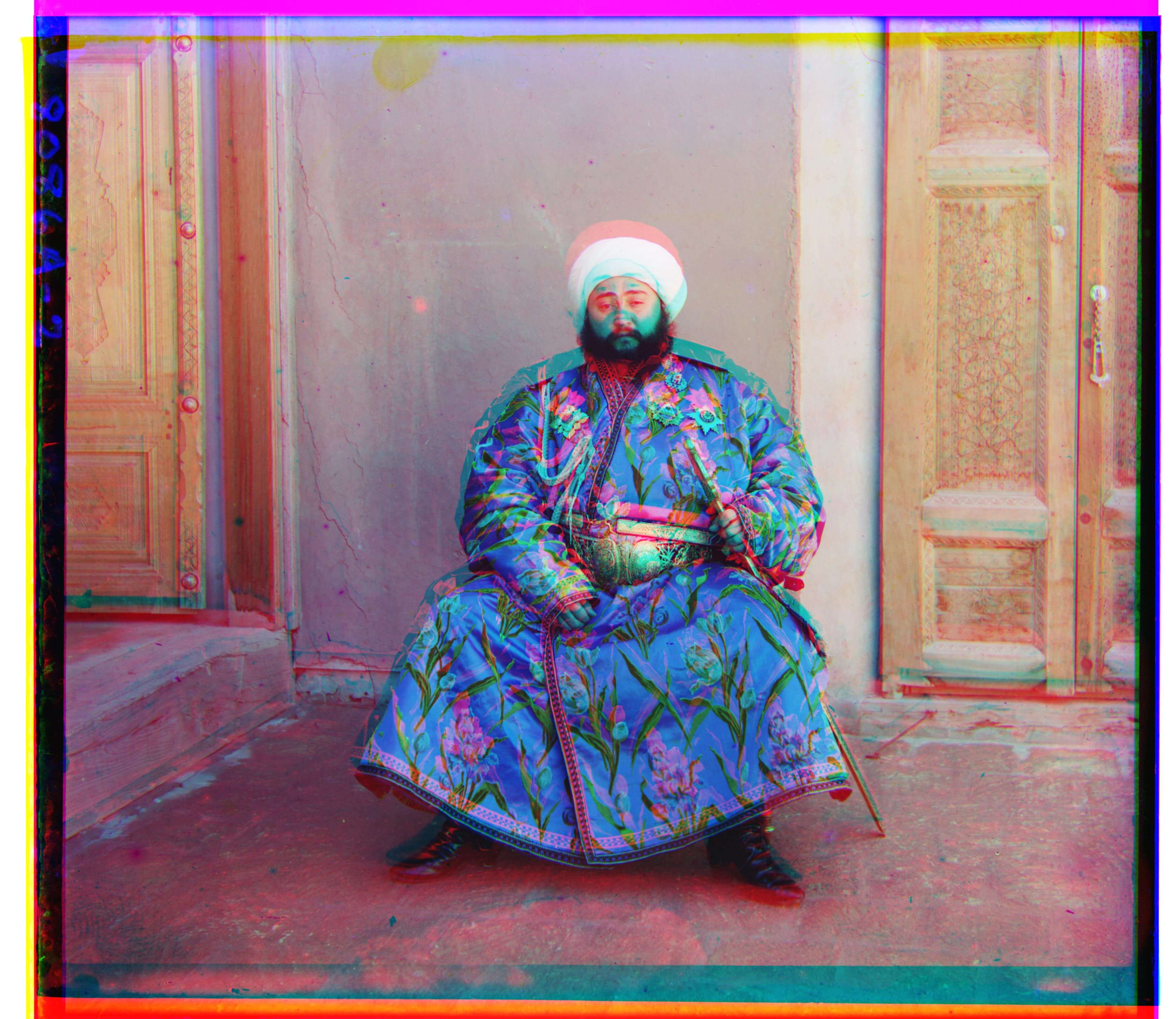
emir.tif
G: [23, 48]
R: [29, 51]

emir.tif
G: [23, 48]
R: [31, 63]

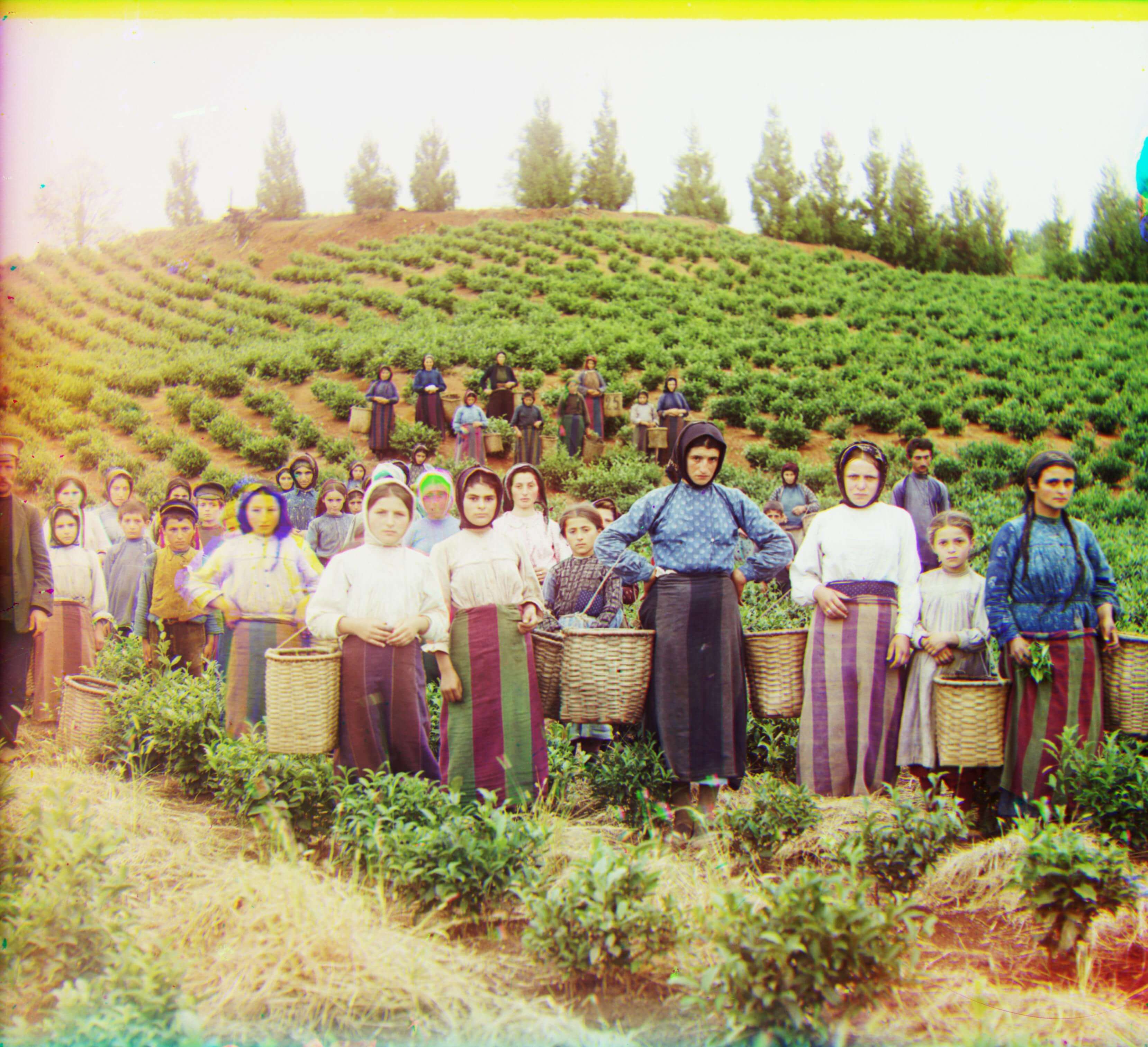
harvesters.tif
G: [19, 59]
R: [17, 124]
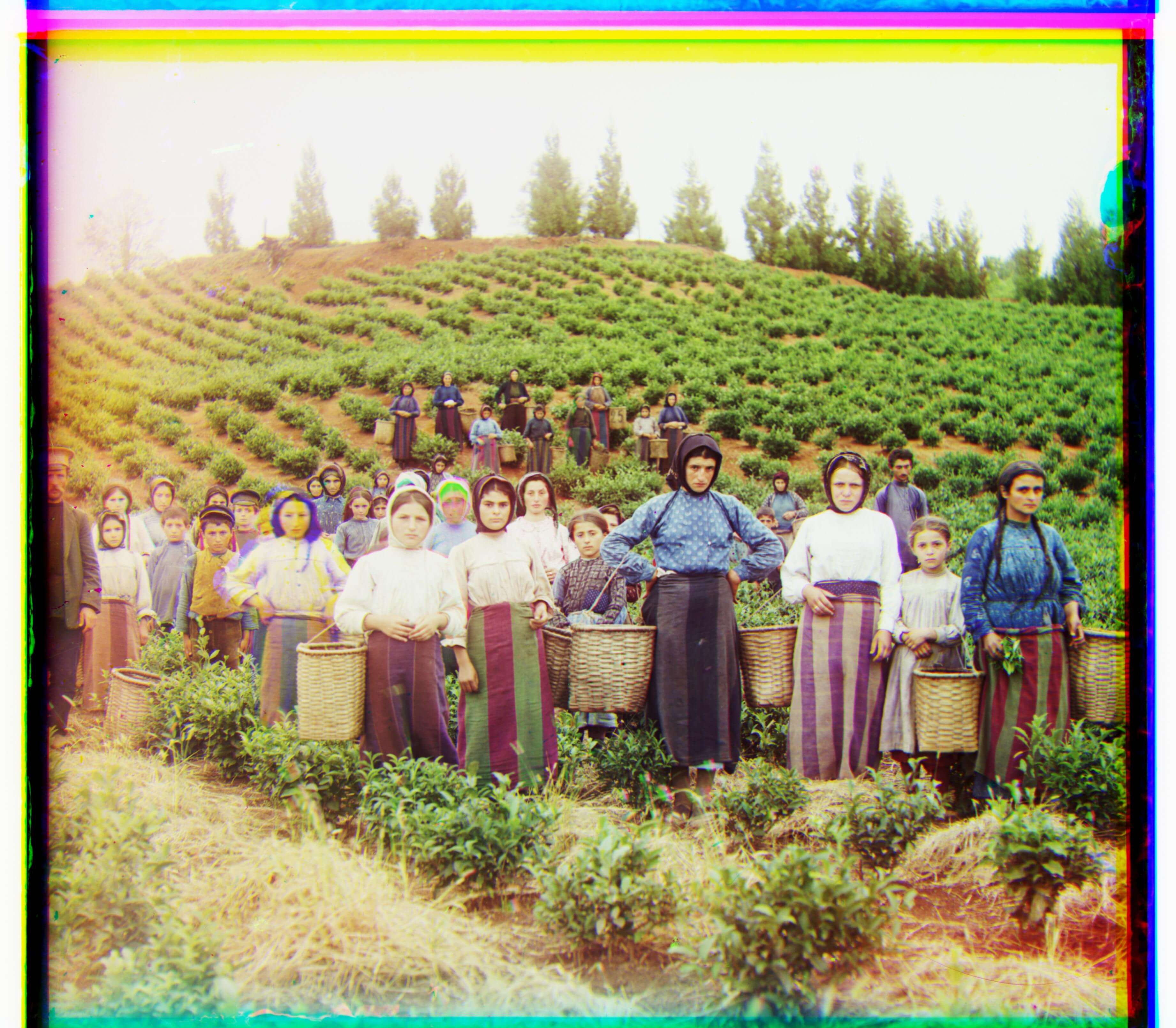
harvesters.tif
G: [18, 59]
R: [16, 123]
icon.tif
G: [18, 41]
R: [24, 89]
icon.tif
G: [18, 41]
R: [24, 89]
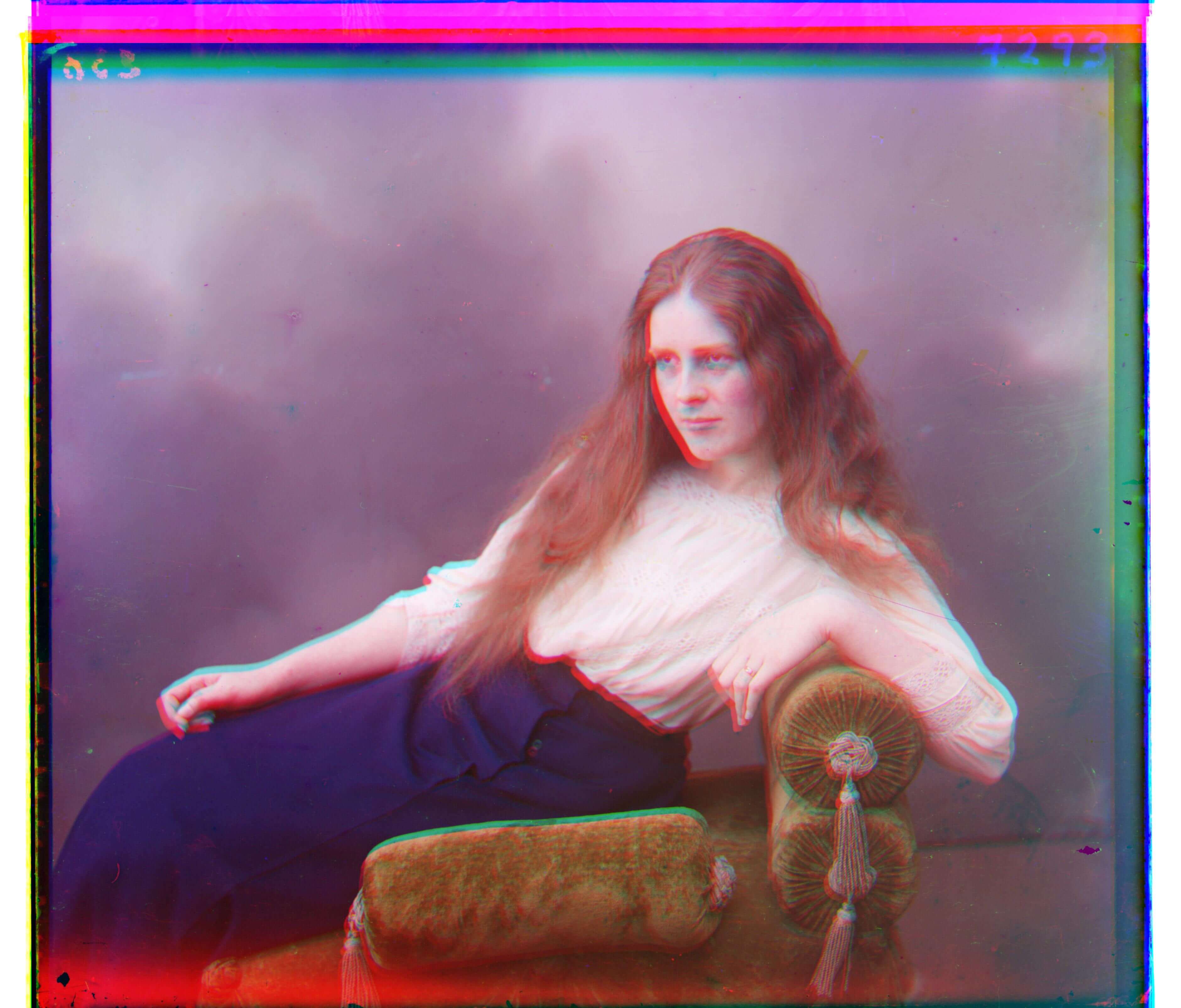
lady.tif
G: [6, 52]
R: [-5, 137]
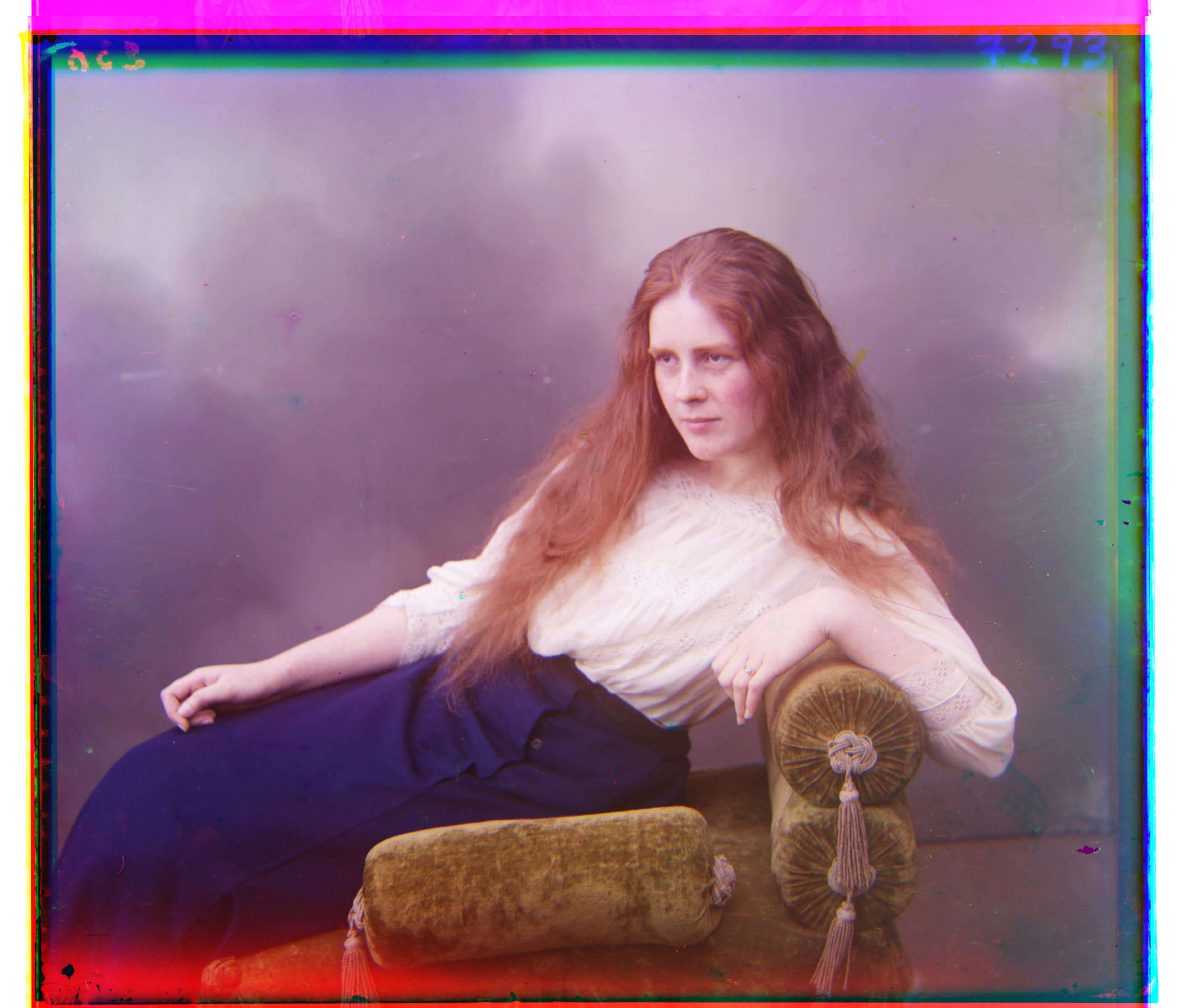
lady.tif
G: [6, 51]
R: [10, 111]
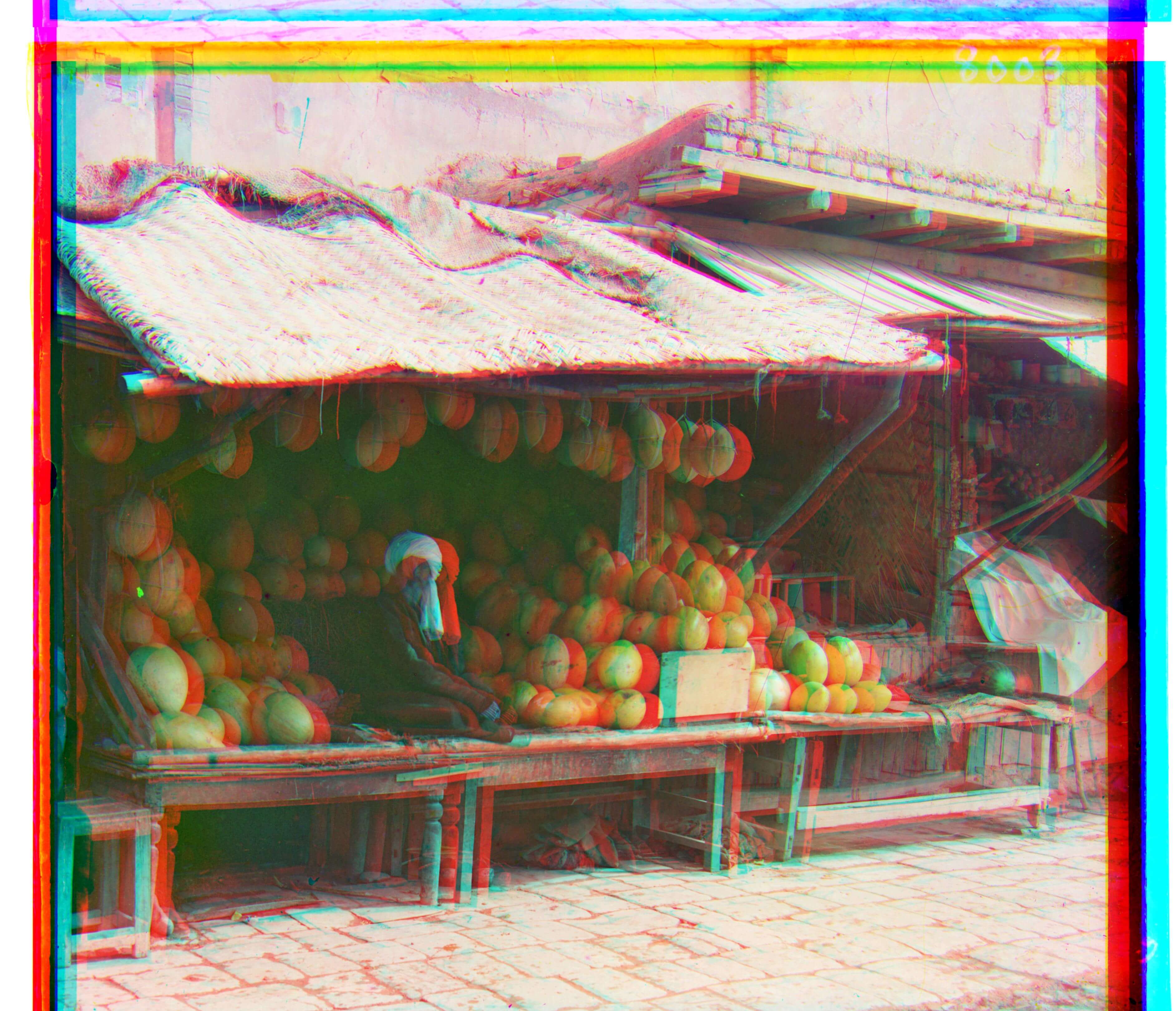
melons.tif
G: [6, 87]
R: [65, 196]
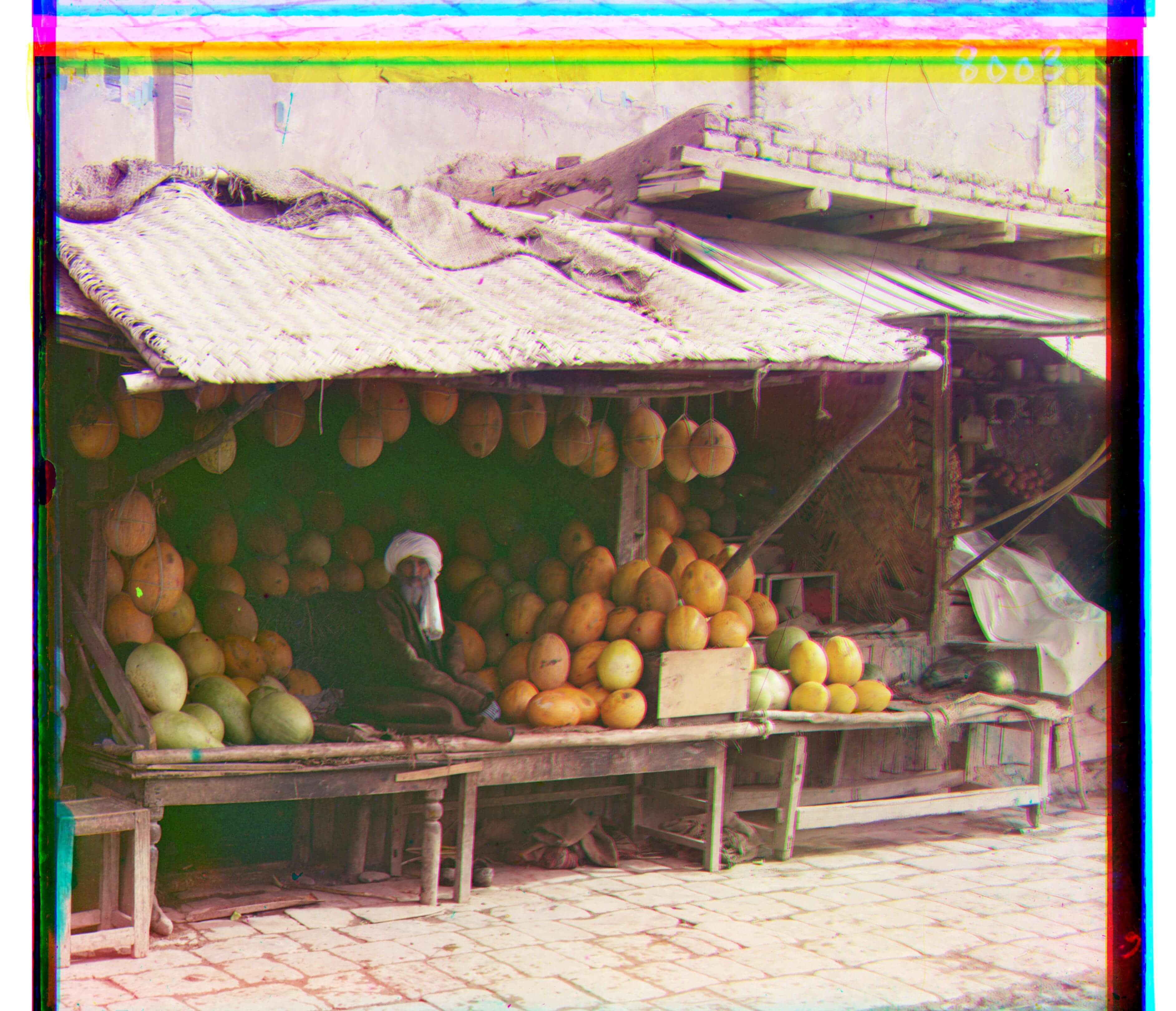
melons.tif
G: [3, 87]
R: [12, 180]
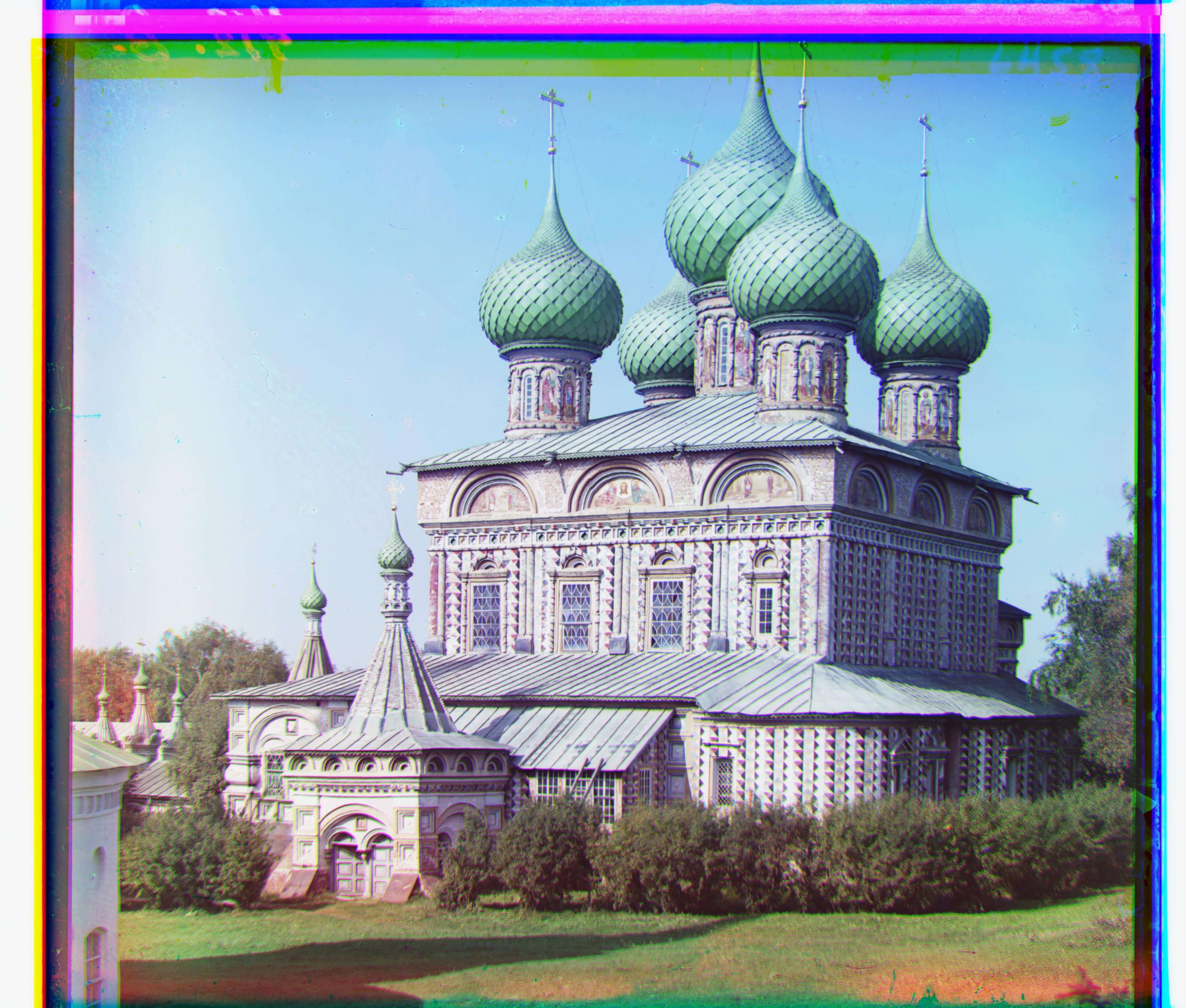
onion_church.tif
G: [26, 49]
R: [37, 107]

onion_church.tif
G: [26, 49]
R: [37, 107]

self_portrait.tif
G: [29, 77]
R: [37, 175]
self_portrait.tif
G: [29, 77]
R: [37, 175]
three_generations.tif
G: [25, 61]
R: [13, 108]
three_generations.tif
G: [15, 49]
R: [12, 108]

train.tif
G: [6, 42]
R: [32, 85]
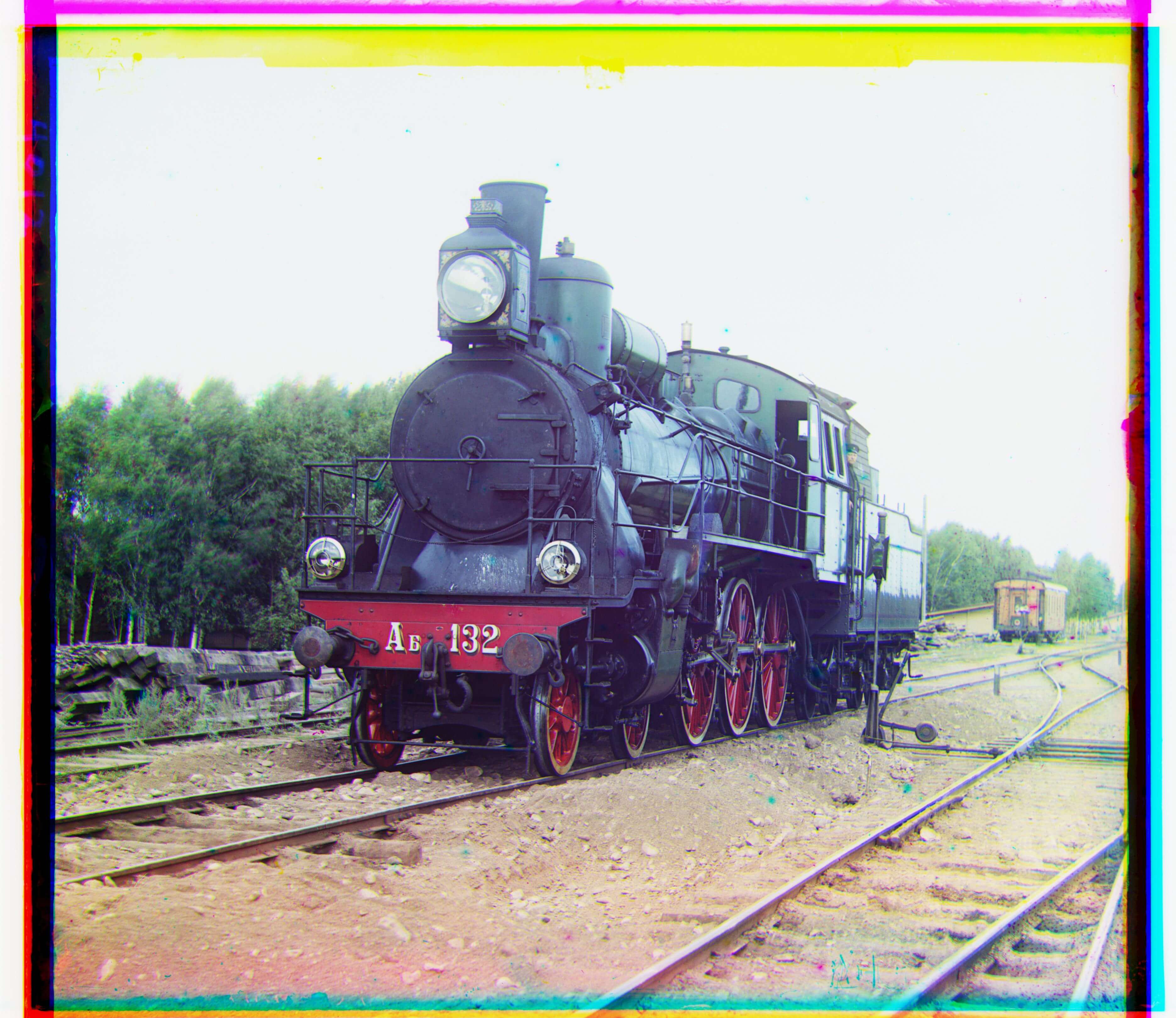
train.tif
G: [6, 42]
R: [32, 85]
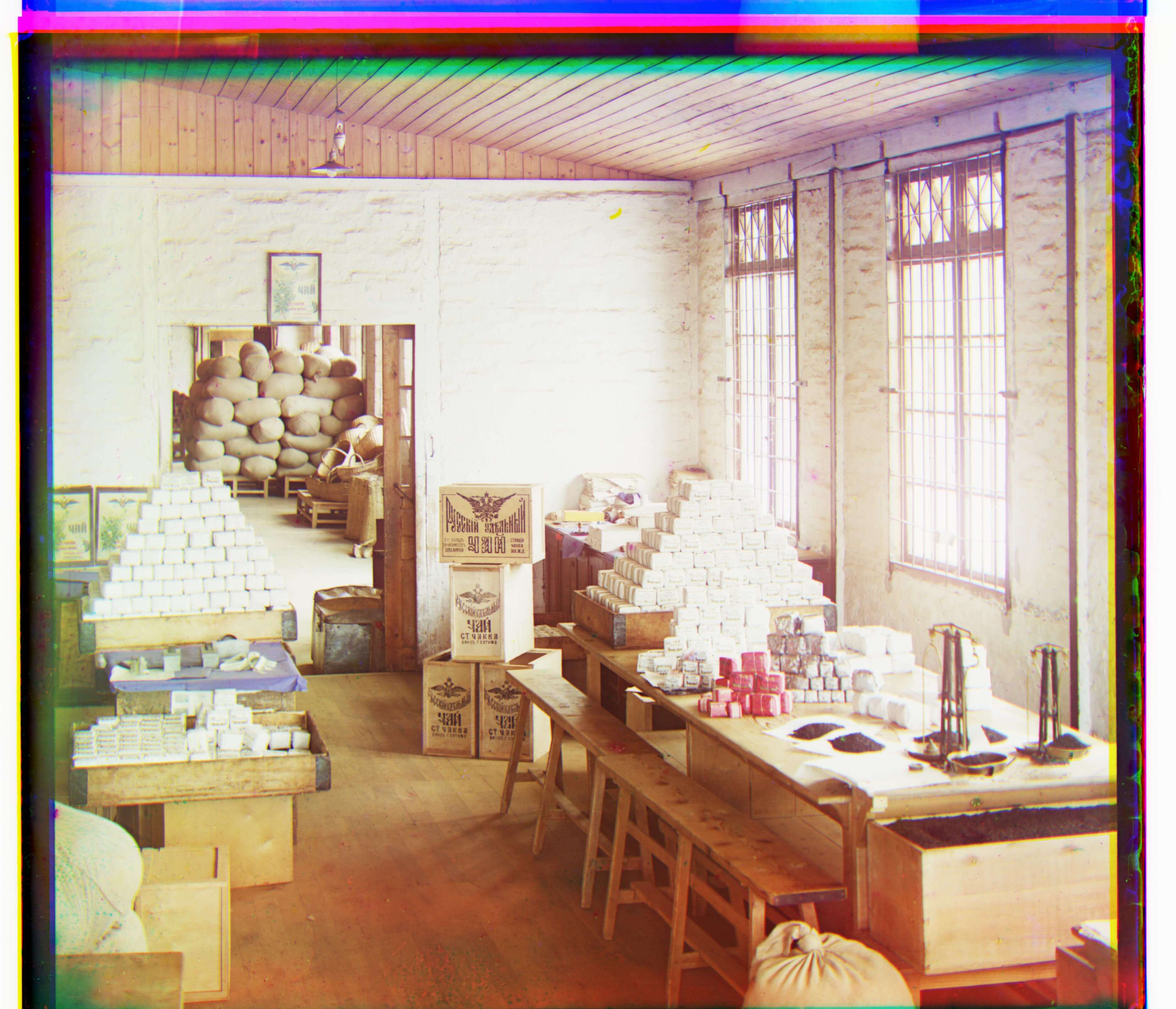
workshop.tif
G: [0, 53]
R: [-11, 105]

workshop.tif
G: [0, 53]
R: [-11, 106]

arch.tif
G: [22, 74]
R: [35, 154]
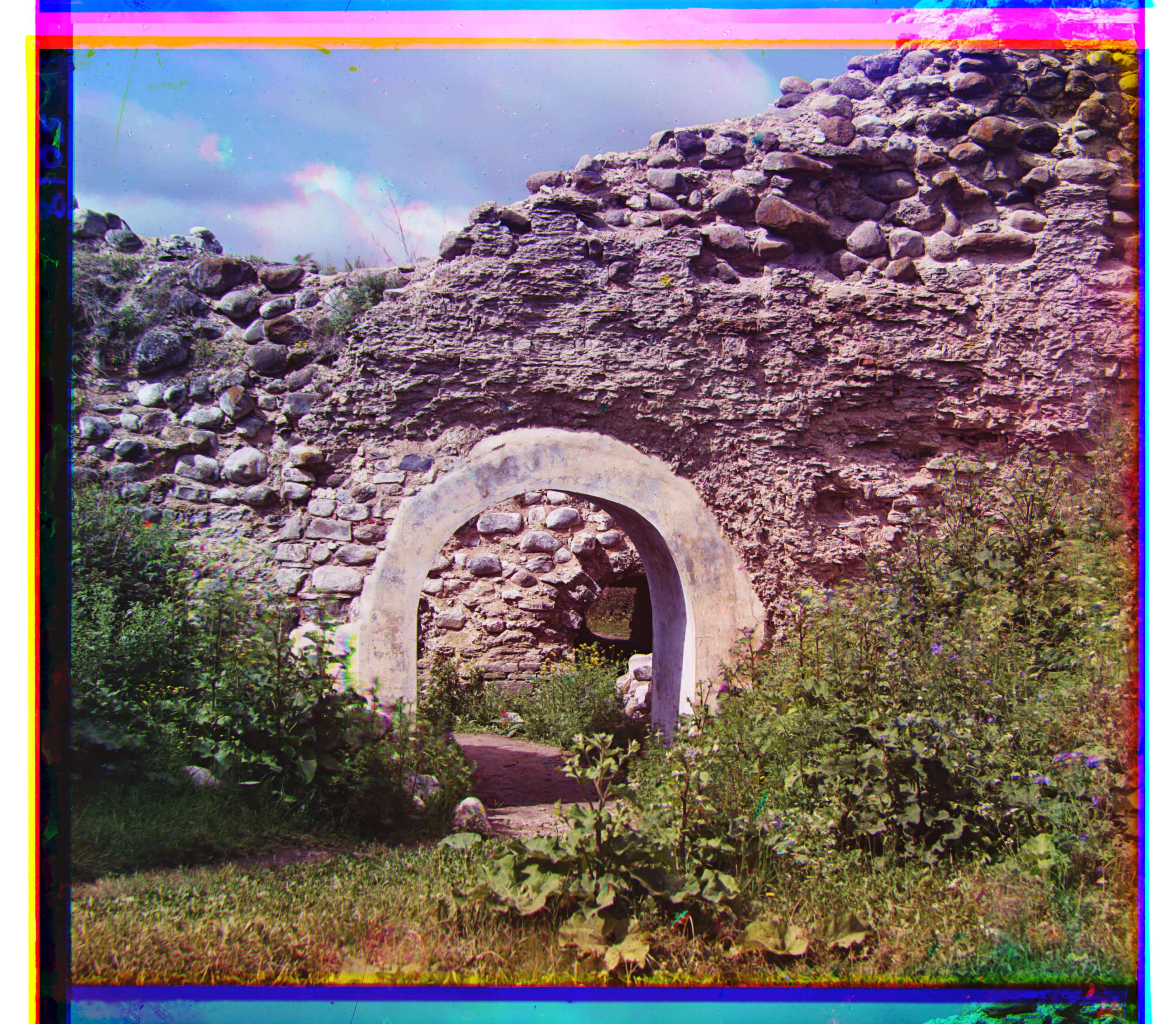
arch.tif
G: [22, 74]
R: [35, 154]

women.tif
G: [10, -13]
R: [20, 12]
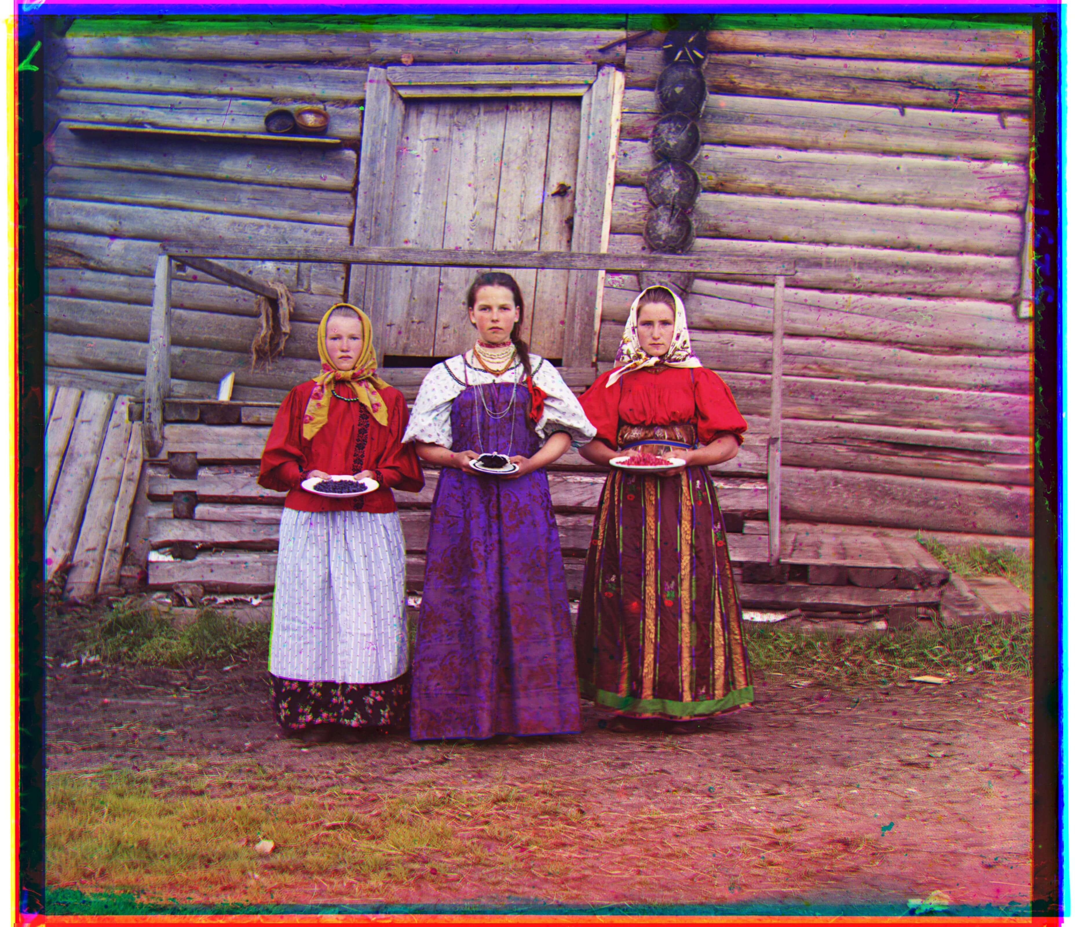
women.tif
G: [10, -13]
R: [20, 13]
There are two things that I want to comment on.
First, the difference between the results for SSD and NCC are not absolutely game-changing,
but NCC does come out on top for images like lady.tif, melons.tif and three_generations.tif.
Specifically, it is easy to notice how much clearer the images are for NCC than for SSD. As
they got similar (or the same) displacement vectors for the other images, we can loosely
conclude that NCC is a better image matching metric than SSD. I believe this is fair because
there is a sizeable trade-off in running time when performing NCC compared to SSD.
Second, emir.tif doesn't look great for both NCC and SSD. However, I was not surprised by
this as there was a fair warning in the project spec about this specific image: "Note that in
the case of the Emir of Bukhara, the images to be matched do not actually have the same
brightness values (they are different color channels), so you might have to use a cleverer
metric, or different features than the raw pixels." The way that I solved this issue was by
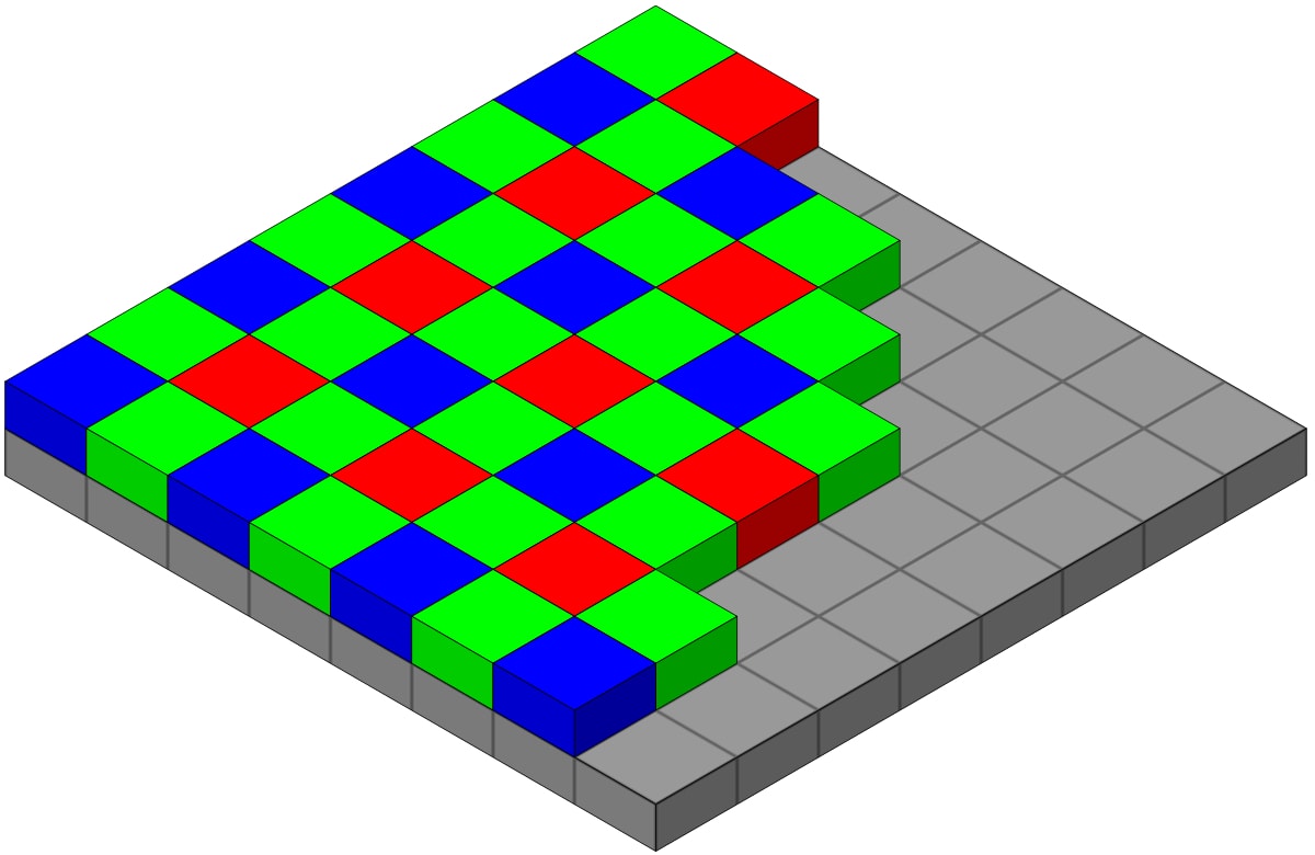
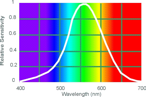
thinking about something I learned about in class: the Bayer filter (top). This filter was
created based off findings summarized by the photopic spectral sensitivity function or PSSF
(bottom). You can see that humans are most sensitive at the middle wavelengths, where the
peak is at green. The spectral sensitivity falls off towards blue and red. As such, the Bayer
filter takes that information into account by giving more emphasis on green.
So, how can we do something similar? We can change the base channel from blue to green! That fixed the problem splendidly (as seen below). Once again, I gave the results below for SSD (left) and NCC (right), and the color channels for the displacement vectors are now blue and red.
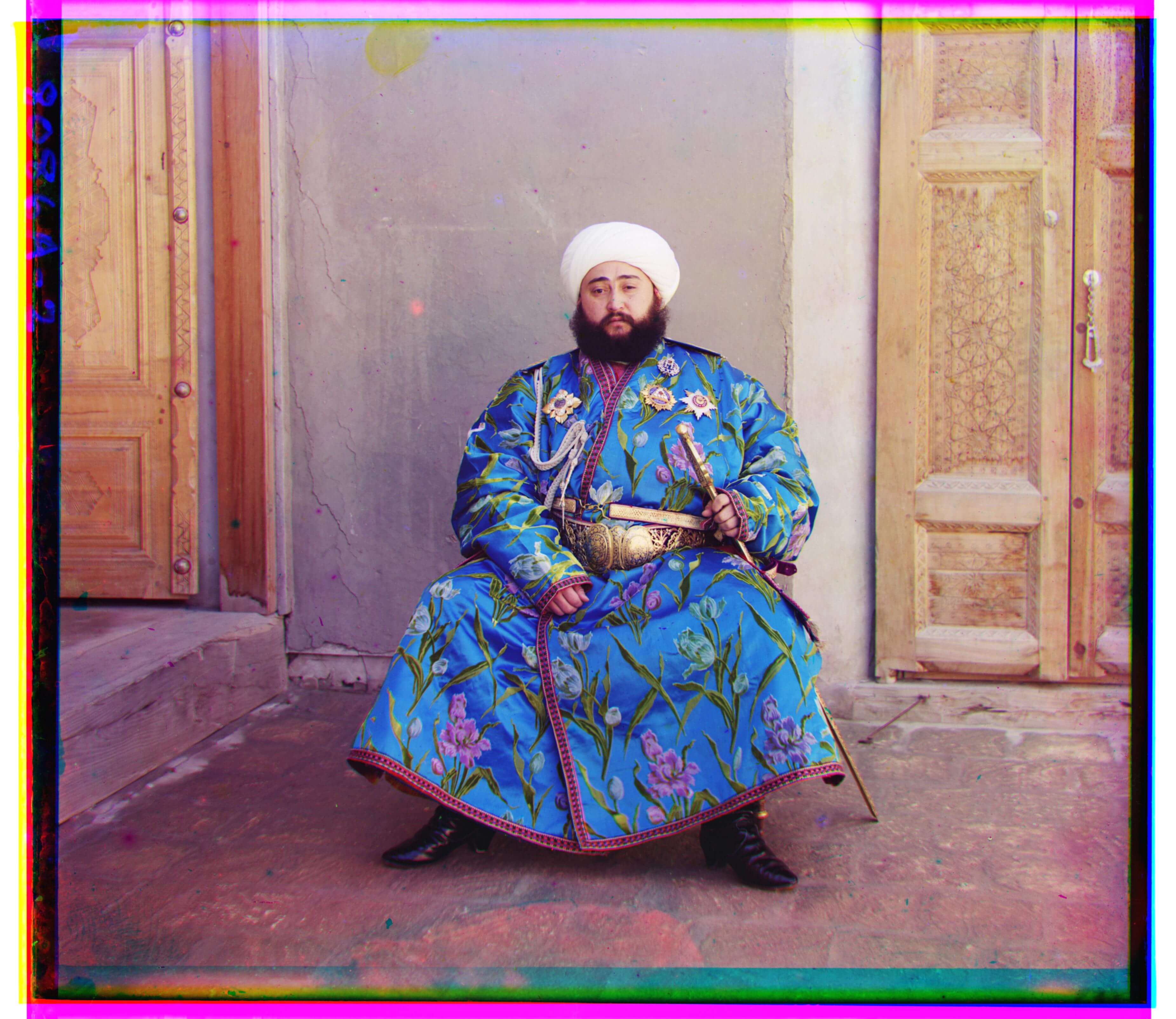
emir.tif
B: [-23, -48]
R: [17, 58]

emir.tif
B: [-23, -48]
R: [17, 58]
harvesters.tif
Old Shape: (3218, 3683, 3)
harvesters.tif
New Shape: (3026, 3317, 3)
melons.tif
Old Shape: (3241, 3770, 3)
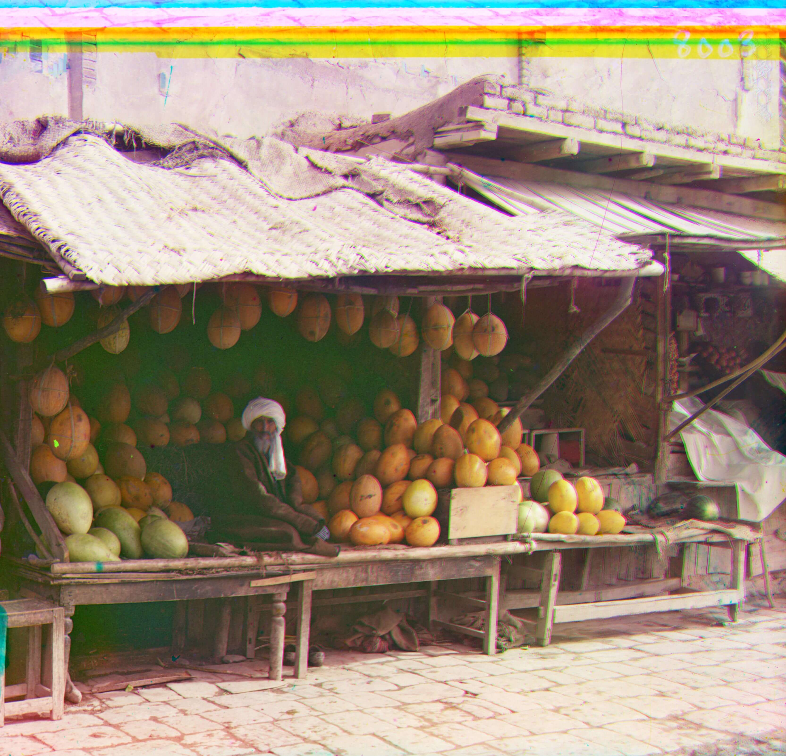
melons.tif
New Shape: (3205, 3330, 3)