Overview
In this project, we colorized images from the early 1900s, bringing to fruition the dreams of Sergei Prokudin-Gorskii. Prokudin-Gorskii photographed various scenes with a unique approach: once with a red filter, once with a green filter, and once with a blue filter. Though he only had a black and white image for each of these captures, we are now able to stitch together these trios of images to produce a full color image of the scene. However, to do so, we must first align the three images, since they are slightly offset. We must then colorize each channel appropriately before stacking to produce the whole colorized image.
Part 1: JPG Images
JPG Approach
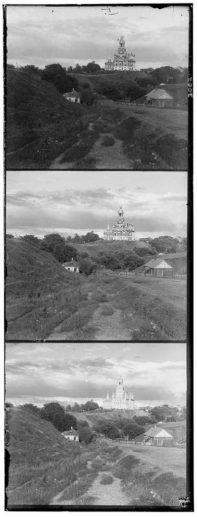
The images are provided by the Library of Congress as three stacked images: blue, green, then red channels. They are not perfectly aligned, and they have obvious differences in intensity in each channel.
|
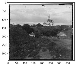
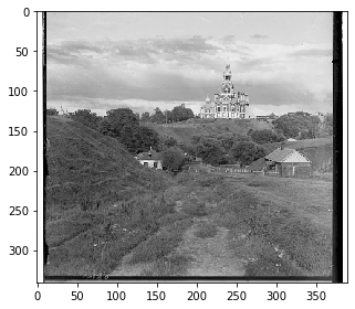
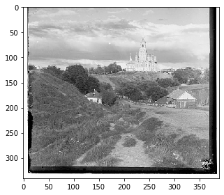
Because jpg images are fairly small, we can run a pretty intuitive approach to the scans. We want to align the images while they are in greyscale. To do this, we split the image into three different ones: blue, green, and red.
|
|
|
To align the images, we choose one to be a stationary template. We can then choose another one of the images and start shifting it around until it lines up well. We know that the images are not terribly poorly aligned, so we do not have to shift it very much. For our purposes, we say that we can shift the image in the x and y directions -8 to 8 pixels. This is to say it can move 8 pixels up, down, to the left, and to the right. For each of these alignments, we check how well the image lines up.
But what is the measurement to say how "well" something lines up? We use the SSD, or sum of squared differences. At each alignment, we take the difference between each pixel, square it (so they're all positive), and then sum across every pixel. In other words, we apply sum(sum((image1-image2).^2)). It's important to note that boundaries are rather iffy, since they are included in our rgb channels but are not meaningful in alignment. Thus we crop out 1/16th of the image on all sides; we are only interested in the real meat of the image at its center.
|
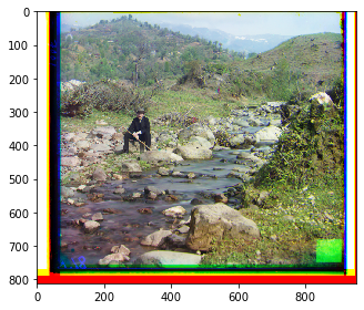
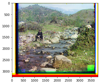
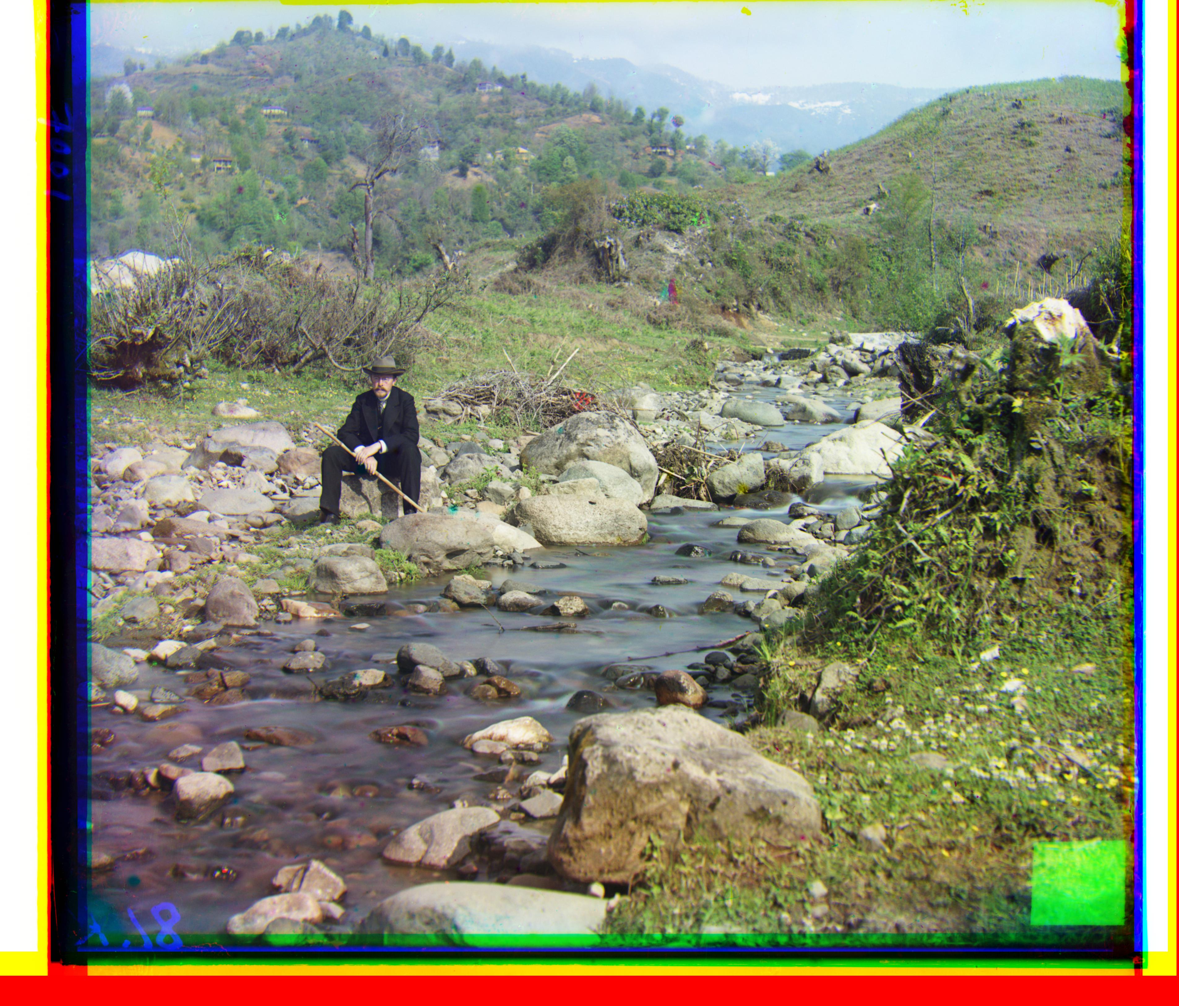
JPG Results
Course Examples
Note in all images, red is used as the reference, so the blue and green offsets are provided. Offsets are provided as (n, m) where n is the offset in the x and m is the offset in the y.
(I apologize to course staff, as I realized too late that the project spec requests us to use blue as the template.)
|
|
|
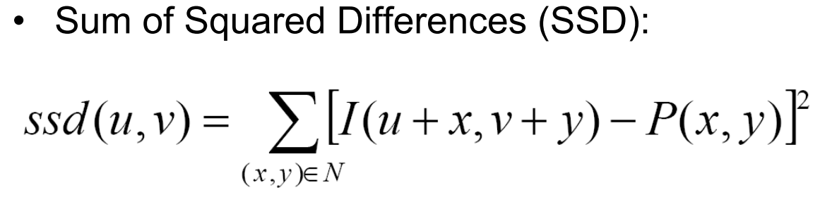
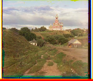
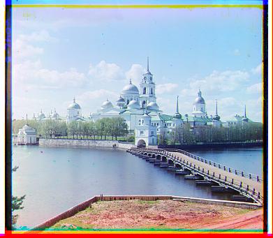
Extra Examples
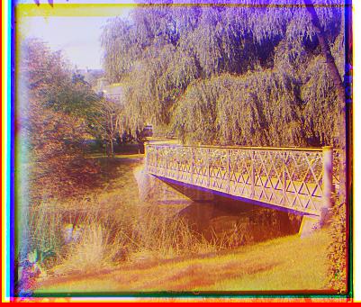
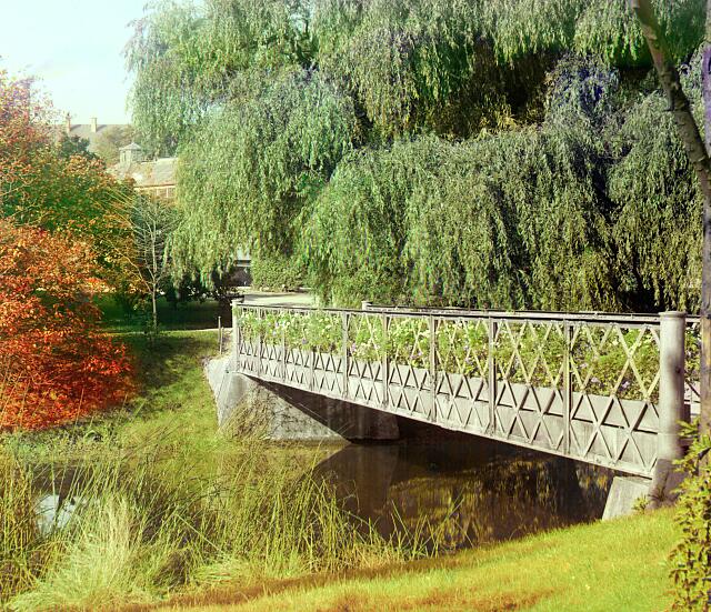
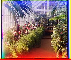
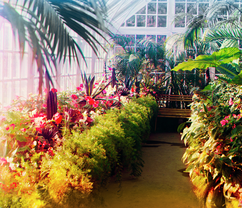
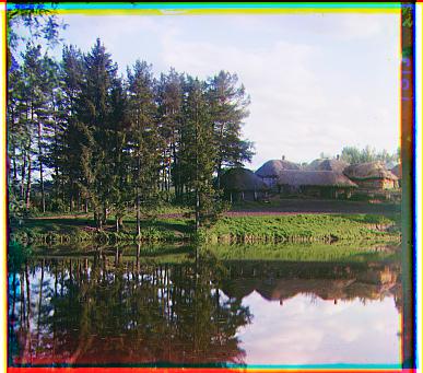
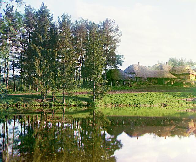
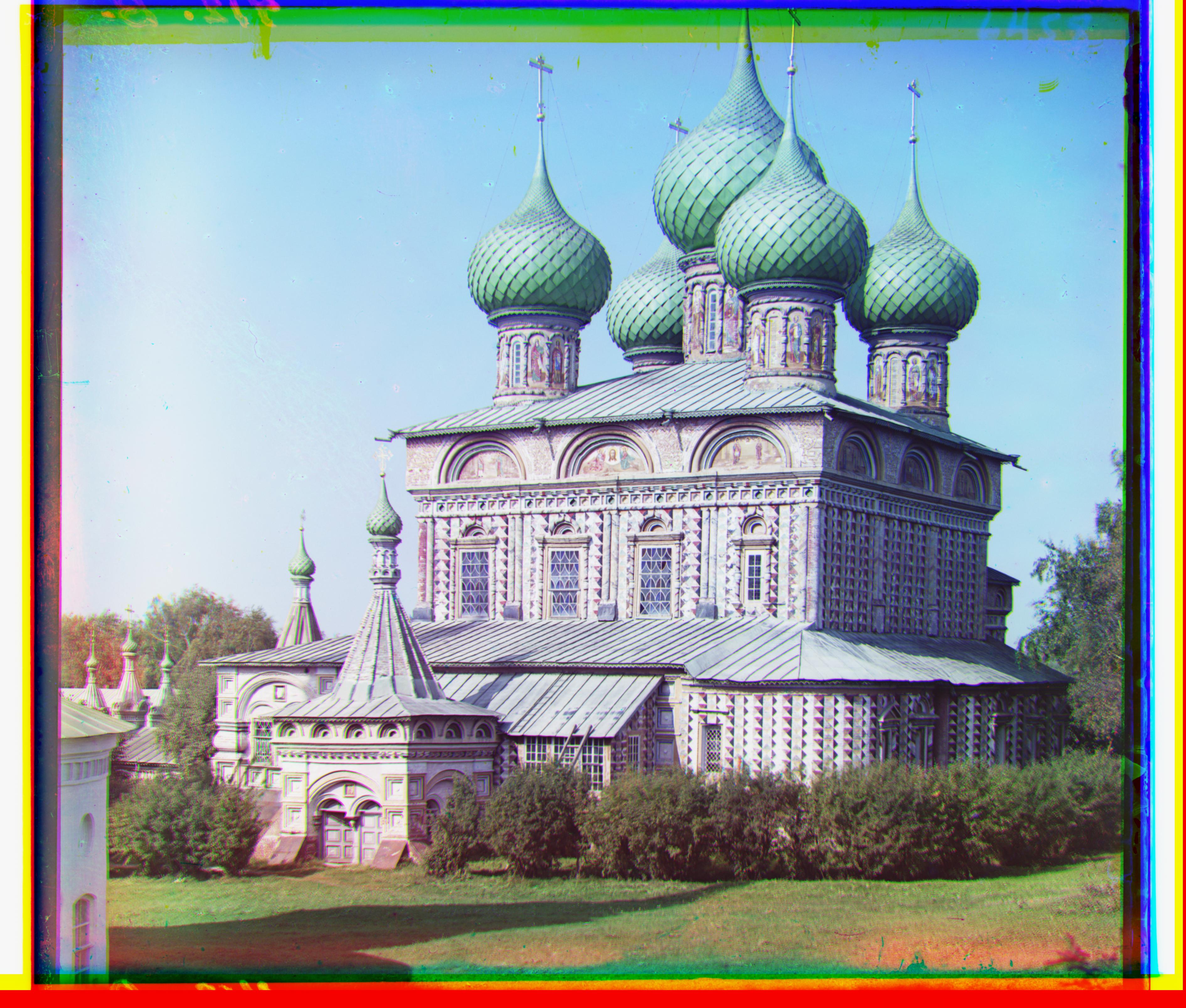
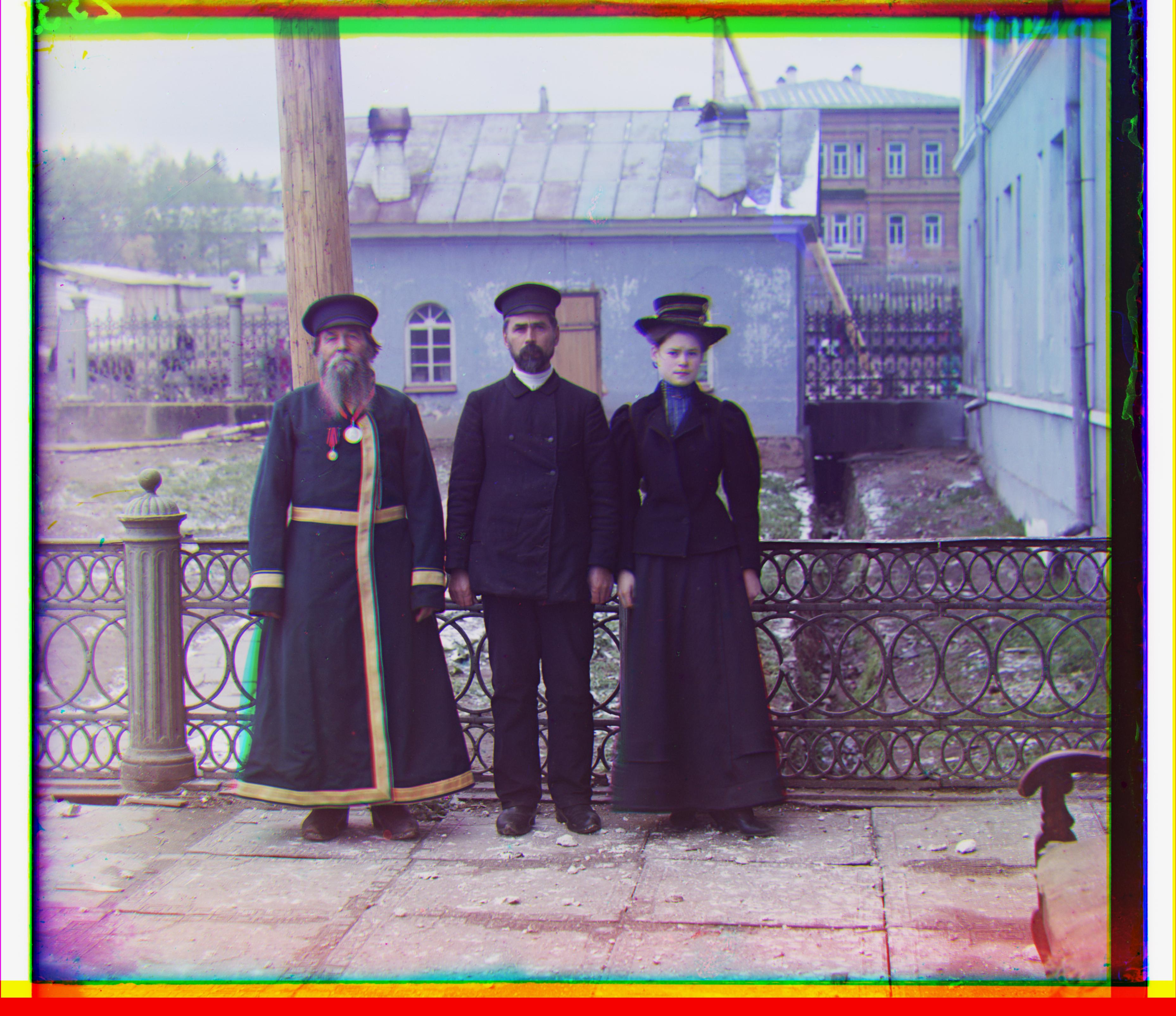
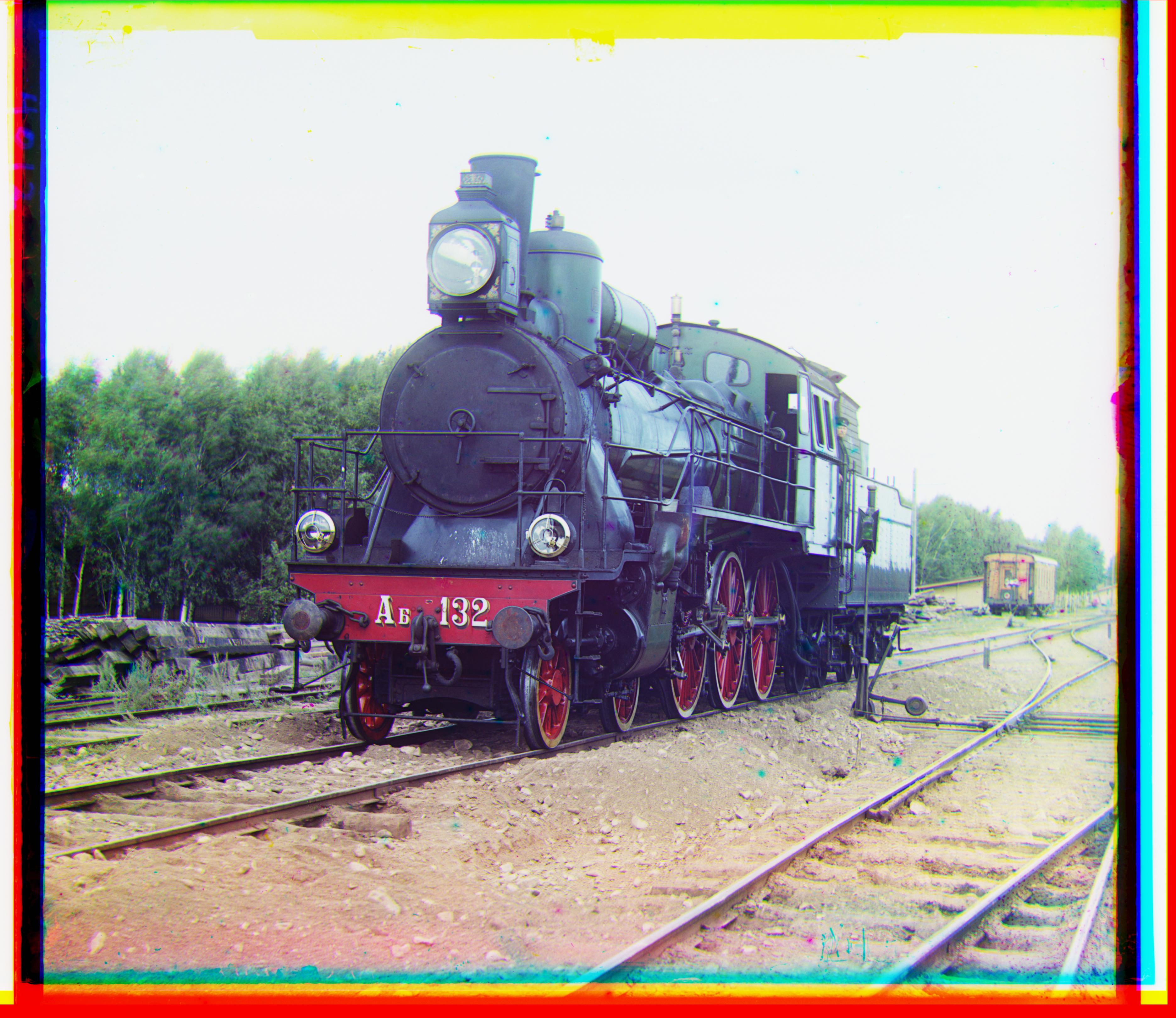
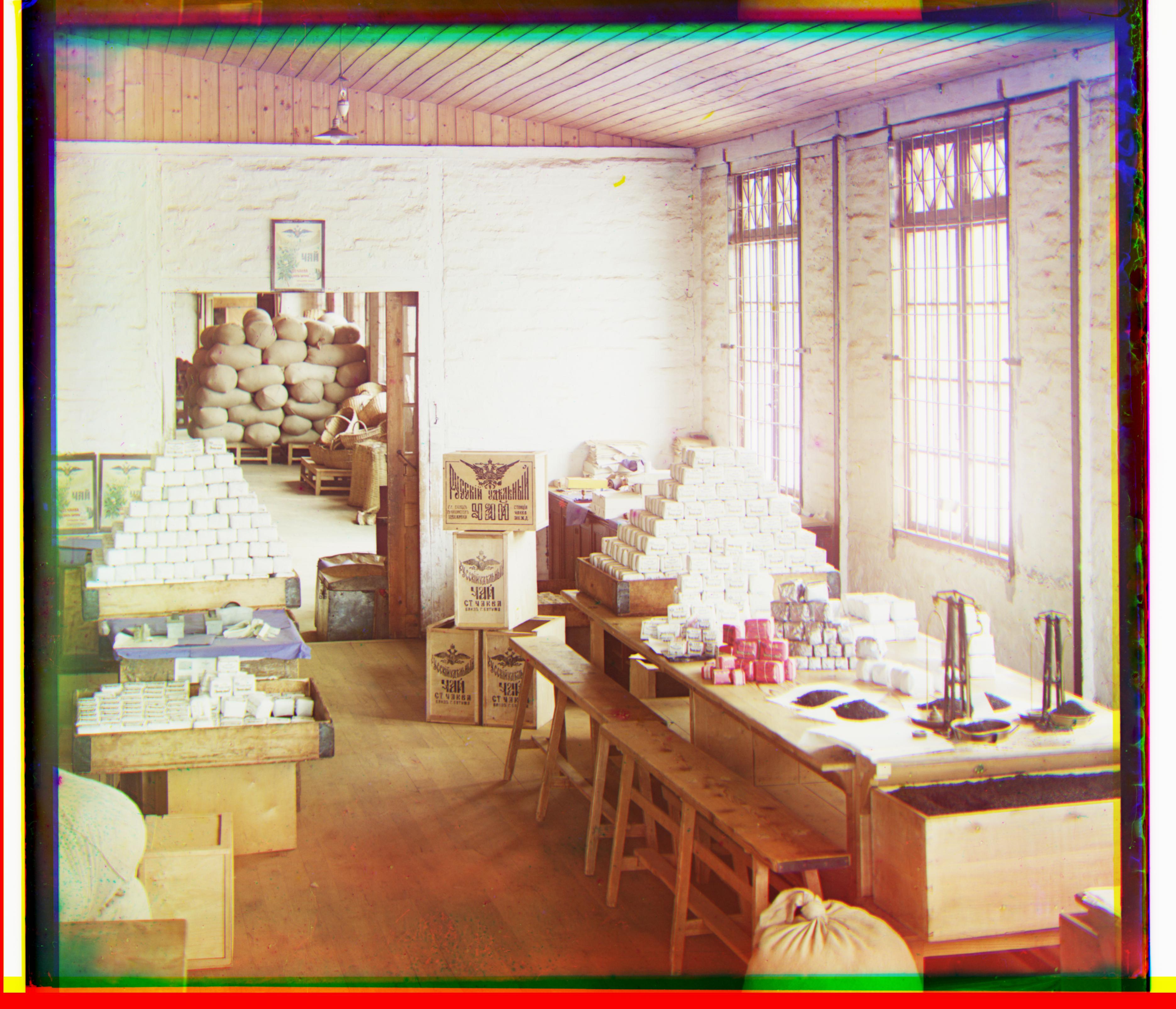
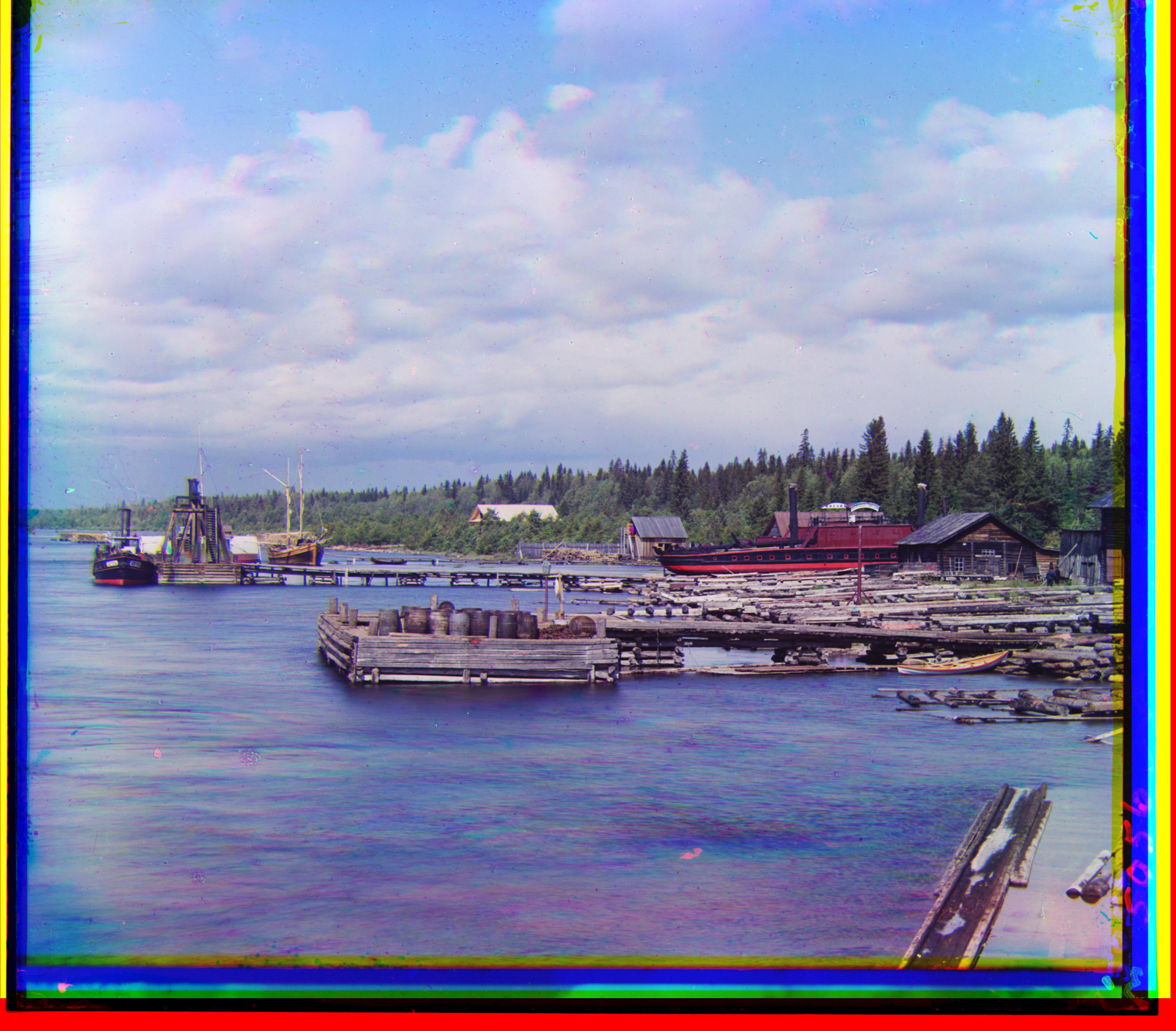
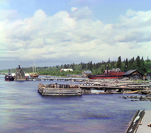
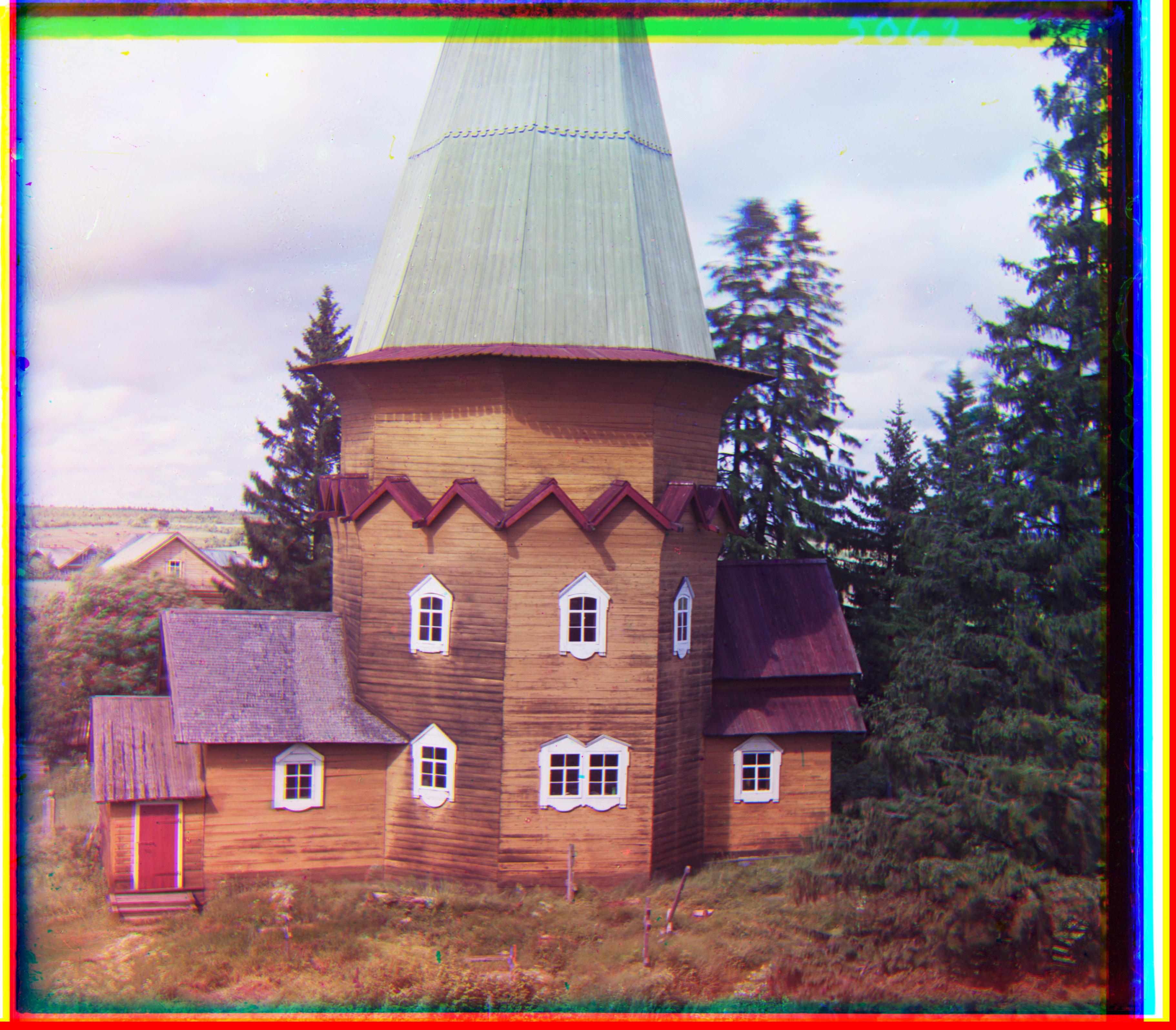
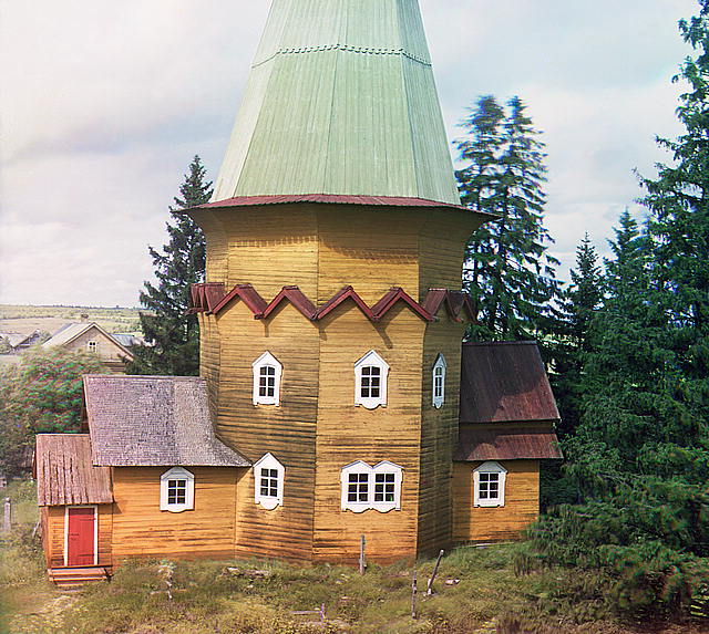
Below are some additional examples. Our colorization is on the left, and there are references from the LoC on the right that are more expertly restored with better adjustments. However, you will note, especially for Little Russia, that our basic approach works reasonably well anyway.
|
|
|
|
|
|
Part 2: TIF Images
2.1: TIF Approach
Our JPG approach only works in a reasonable amount of time because JPG images are compressed and reasonably small. However, for large image formats, like TIF, we cannot possibly exhaust every possible alignment pixel-wise. Because there are so many pixels in a high resolution scan, it's also hard to say what a reasonable neighborhood of search is. Consequently, we must apply a different approach. Thankfully it's not too different from what we've already done!
In order to recycle some of what we've done, we create a "pyramid" of images. We take the original image and downscale it by factors of 2 repeatedly. At each step the image becomes coarser--which is to say, lower resolution. We build the image pyramid and then start at the top of it with the coarsest image. We can then run the JPG approach since the image is small. Once we've aligned this coarse image, we have a better idea of where to look in the next image down the pyramid: twice the offsets that minimize the SSD. (We need a factor of 2 times since the images are scaled by a factor of 2.) So instead of searching exhaustively, we have a smart "starting point" to examine the neighborhood around it. Basically, we take "guesses" from coarser images and then update our guesses at higher resolutions. The whole process takes roughly 1 minute per TIF image. For an old machine like mine, that's pretty good!
You can see below the progression of "guesses" that gets sharper (more aligned) with each iteration.
|
|
|

|
|
|
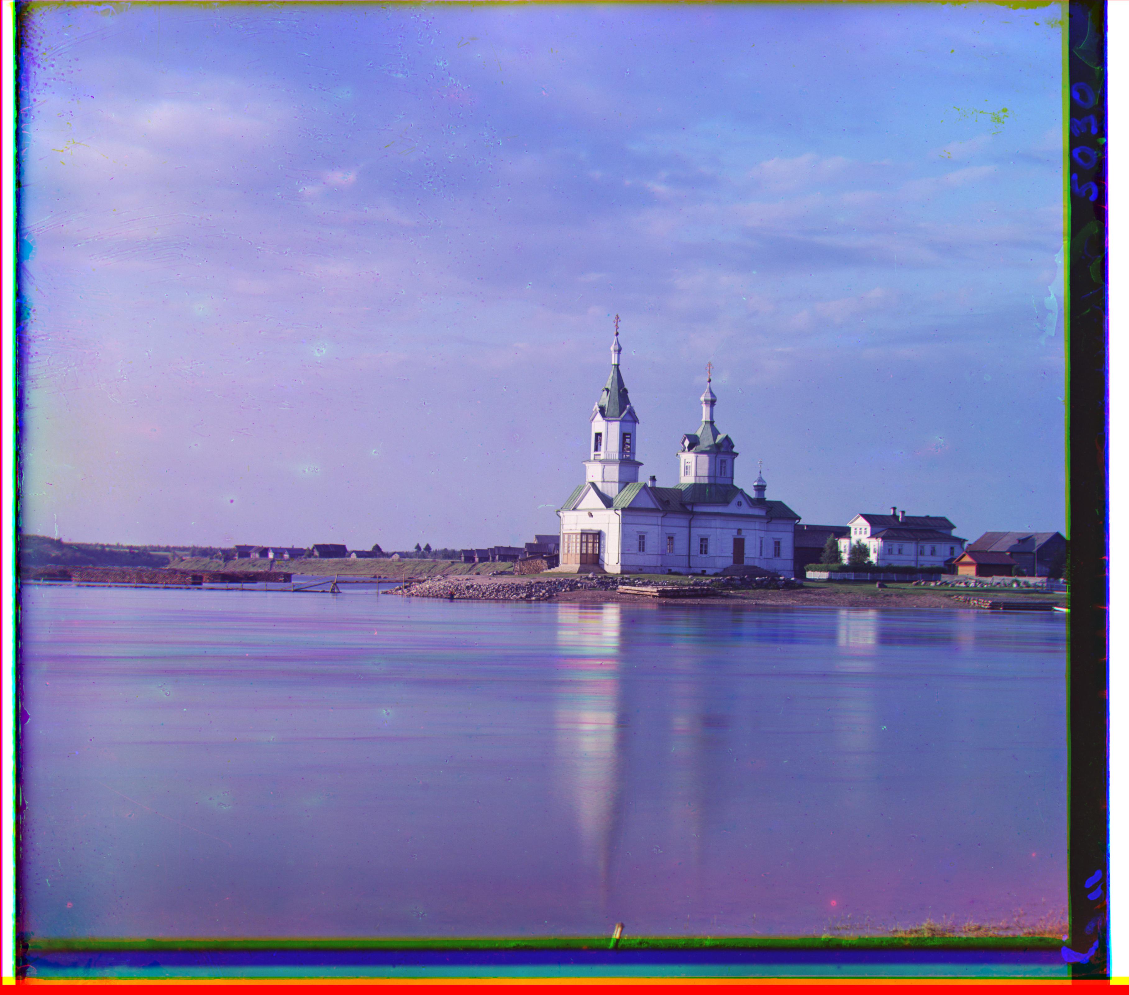
2.1 TIF Results
Course Examples
|
|
|
|
|
|
|
|
|
|
|
|
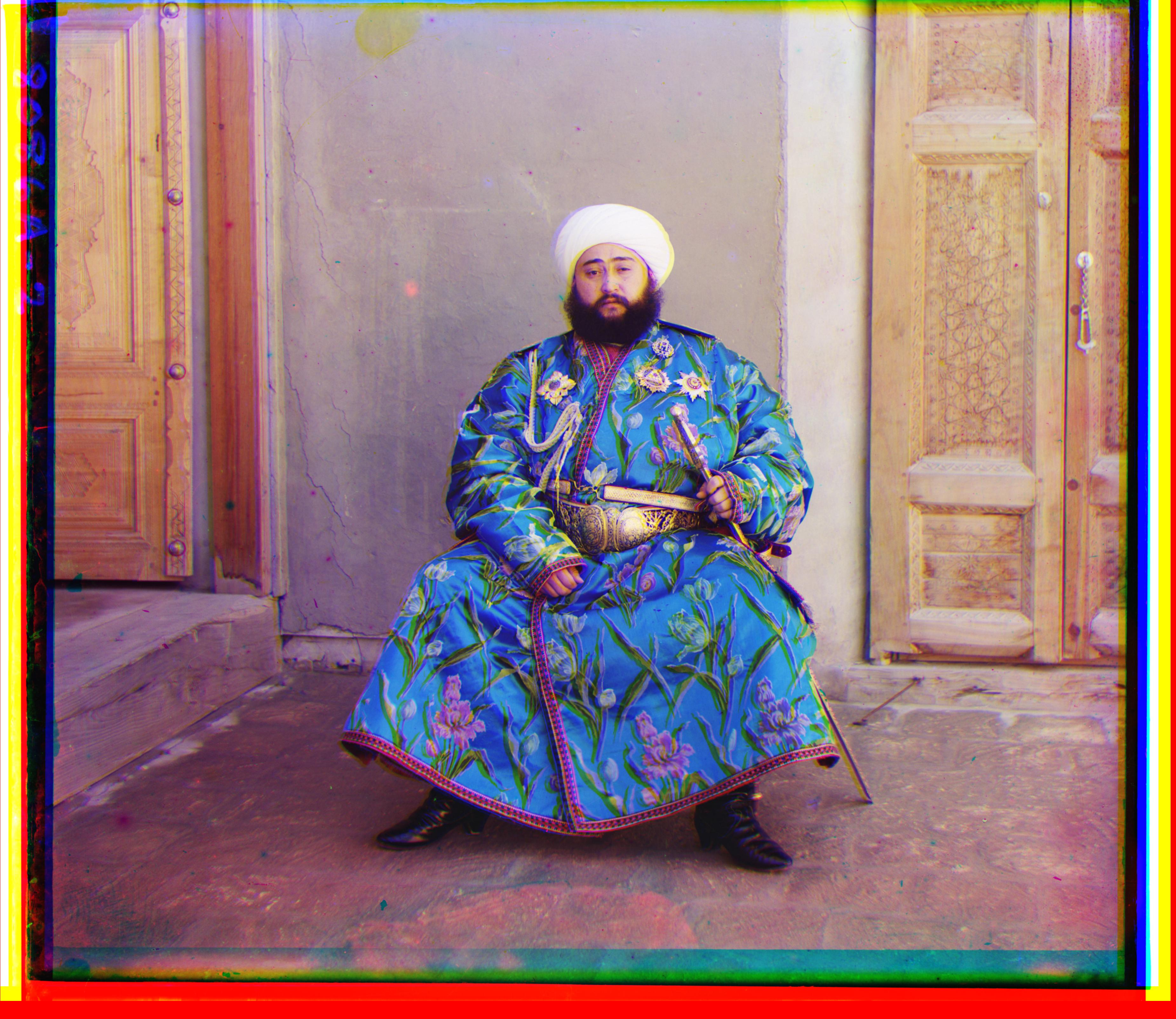
Note in Figure 10, Emir, that the green channel is just slightly offset, though it is not apparent at a quick glance. This is because the brightness on the channels are different, so it is hard to match with our naive SSD. That being said, it does pretty well overall.
Extra Examples
|
|
|
|