

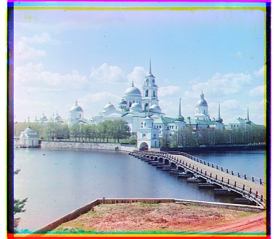
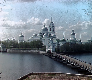
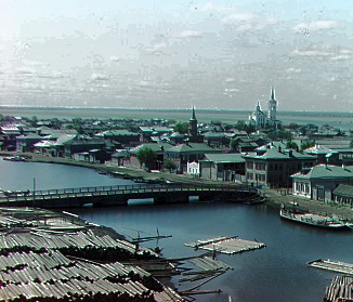
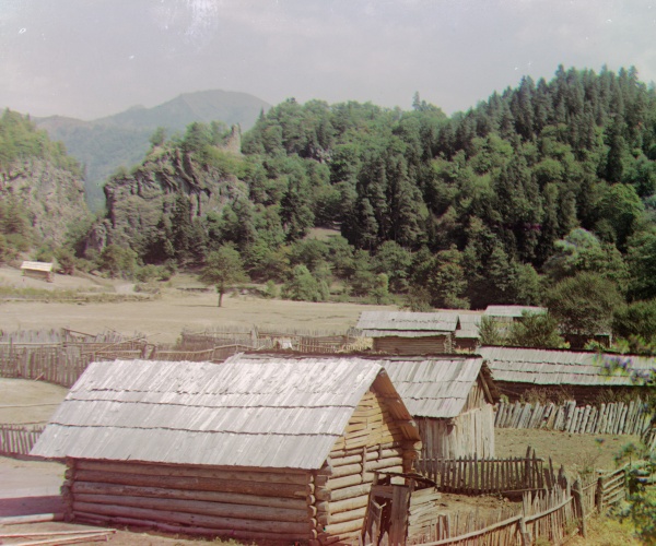
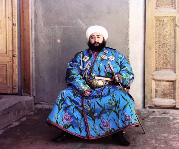
This project aims at recovering a colorful photograph given three distinct exposures of the same scene with a green, blue, and red filter. These photographs were taken by Sergei Mikhailovich Prokudin-Gorskii in the early 1900s and were kept in the Library of Congress. Note that these three photographs might be slightly shifted and the scene might change as well. Thus, the colorization process will involve image alignment by searching the displacement over image pyramids, as well as further refinements such as auto white balancing, auto contrast and auto cropping.
Given two images of the same scene with slight shift, we can fix one image and move the other horizontally and vertically to find a perfect match. To measure the quality of the alignment, two similarity functions are utilized.
Sum of Squared Differences (SSD) is the sum of squared differences per pixel between the two images. However, since the images were filtered by different color filters, the brightness may be different on the same location.
Normalized Cross-Correlation (NCC) can be viewed as the cosine similarity between two flattened images. In my implementation, the flattend images are first subtracted by its mean pixel to alleviate the impact of brightness difference.
Further, since there exist black edges for the original images, and moving the image by
np.roll will yield a disaligned row or column at the last row or column of the image,
the metrics should only be applied on the central part of the image. This is done by automatic
cropping, which will be described later. In addition, applying the metrics on edge images
rather than the original images sometimes bring better results.
The above computation of SSD and NCC are time-consuming when they are applied to a high resolution image. What's more, finding the optimal alignment requires to iterate over a certain range of pixels, and the range will be large for high resolution images. Thus, constructing an image pyramid for alignment is necessary to reduce computation. The high level pyramid image will have lower resolution, thus faster for every single similarity computation. Since the displacement of the high level pyramid will be mapped to the original image and the higher the level, the bigger the displacement. Thus, the displacement can be achieved by mostly the highest and the second highest levels, and the lower levels will finetune the coarse displacement. So we can only search in a small range for the low level images since they consume a lot of time for computing the similarity metrics due to their high resolution without worrying about insufficient search range.
In my implementation, I used a simple heuristic to decide the search range for a given image, that is the product of the image size and the search range size should be almost identical across different pyramid levels. The value of the product is manually set such that the average runtime for each image is around 30 seconds.
flops = 30 * 30 * 400 * 400
displ_thresh = int(np.sqrt(flops / imga.size) / 2) + 1
displ_range = np.arange(-displ_thresh, displ_thresh + 1)
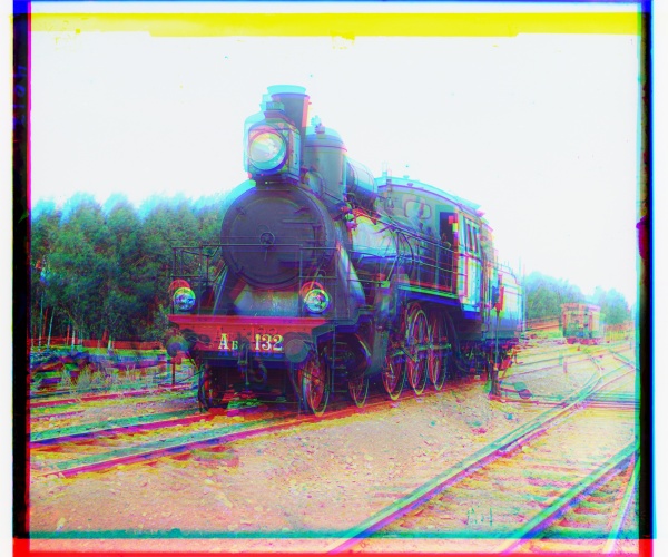
So far, the salient objects can be well colorized via the above process. However, there still exists several problems:
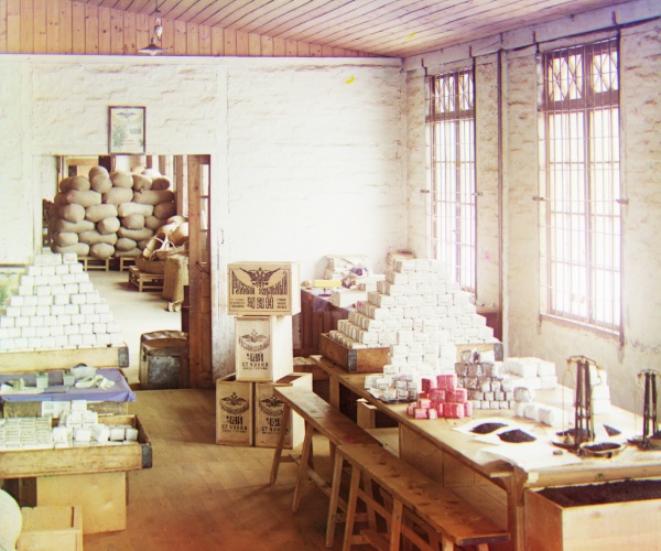
From the results obtained in section 2.1, we can find that the original images contain black edges and the final results contain abnormally colored edges, even when the black edges are cropped at the beginning (see the image for NCC w/ auto cropping). Thus, auto cropping should be applied twice for preprocessing and postprocessing.
Since the edges are usually vertical or horizontal, we can simply apply a high frequency filter (e.g. Canny filter) to yield an edge image and then detect the vertical and horizontal edges. Given that the edges only appear on the border of the image, we can restrict the search range to avoid clipping the image too much. I tried using Hoffman transformation to apply line detection on the edge image at first, however, since the edges may contain discrete pixels and stacking morphology operations and Hoffman line detection can be time consuming, I used a simple way to detect horizontal and vertical edges instead. Basically I just collect the size of edge points and compare it with the height or width of the image to decide whether this line contains an edge, and also I take the edge points on its neighbor lines into consideration. The implementation is shown below.
def remove_boundary(img):
    img = cv2.Canny(img, 50, 150, apertureSize=3)
    border_thresh_y = img.shape[0] // 20
    border_thresh_x = img.shape[1] // 20
    minLength = min(img.shape[0], img.shape[1]) // 10
    bandwidth = 2
    top, bottom, left, right = 0, img.shape[0], 0, img.shape[1]
    for y in range(bandwidth, border_thresh_y):
        if np.sum(np.max(img[y-bandwidth:y+bandwidth], 0)) > minLength:
            top = max(top, y)
    for y in reversed(range(img.shape[0] - border_thresh_y, img.shape[0] - bandwidth)):
        if np.sum(np.max(img[y-bandwidth:y+bandwidth], 0)) > minLength:
            bottom = min(bottom, y)
    for x in range(bandwidth, border_thresh_x):
        if np.sum(np.max(img[:, x-bandwidth:x+bandwidth], 1)) > minLength:
            left = max(left, x)
    for x in reversed(range(img.shape[1] - border_thresh_x, img.shape[1] - bandwidth)):
        if np.sum(np.max(img[:, x-bandwidth:x+bandwidth], 1)) > minLength:
            right = min(right, x)
    return [top, bottom, left, right]
Apparently Hoffman line detection fails to clip the yellow cluster on the upper boundary from the image while my simple strategy successfully clips it. In addition, running Hoffman line detection on this image costs 30.23 seconds, while my simple strategy only consumes 22 seconds.
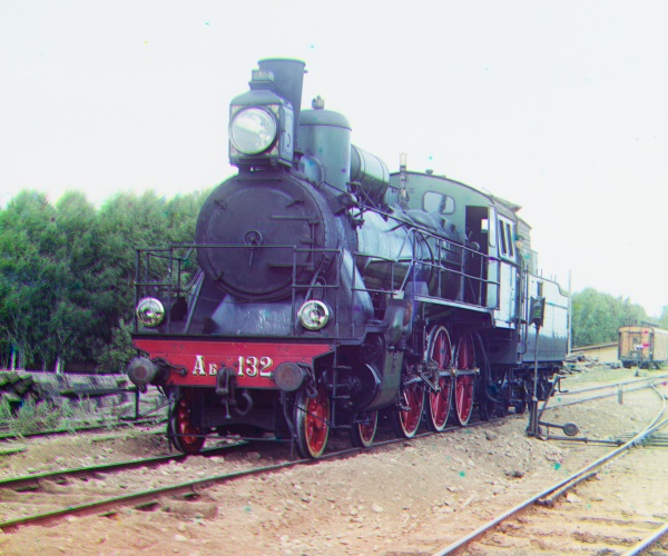
In addition to cropping the abnomally colored edges again at the first step of postprocessing, to make the image looks better, I tried the following operations during postprocessing.
I tried three methods for auto contrast:
The first two methods by normalizing different color channels is of nuance difference, though normalize on the V channel yields very slightly darker image. However, by applying histogram equalization on the V channel yields a very different result, and from my perspective, I prefer the last one since it seems to be more realistic.
I make a simple modification upon the traditional white balancing algorithm under the lightest pixel should have the highest grayscale value assumption. First I convert the image to grayscale and find the top 10% lightest pixels as the light pixel candidates. Then for each channel, the maximum pixel value among those light pixel candidates should be mapped to 255. This modification enables the lightest pixels to be different among different channels. The results with and without auto white balancing is shown below (without other postprocessing). With AWB, the sky in the image seems to be clearer since these light pixels are adjusted.
Given the results of auto contrast via histogram equalization, the lightness of the picture is lower than the original. Thus, I want to adjust the lightness of the image to make it looks better. So I decide to use Gamma Correction to adjust the grayscale values non-linearly to preserve the original color structure of the image while lighting the image up.

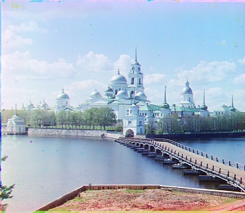
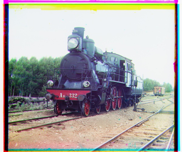
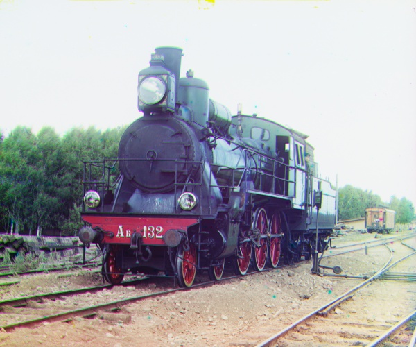
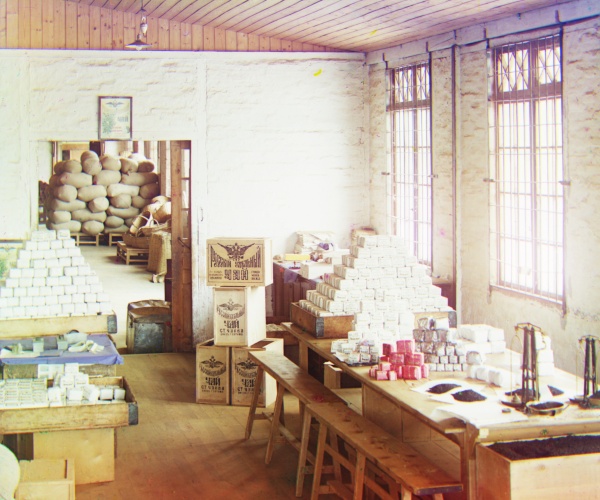
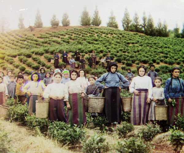
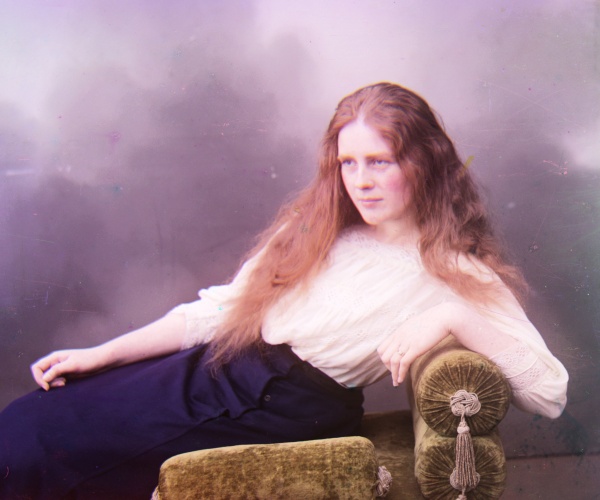
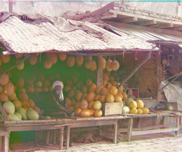
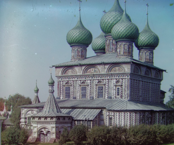
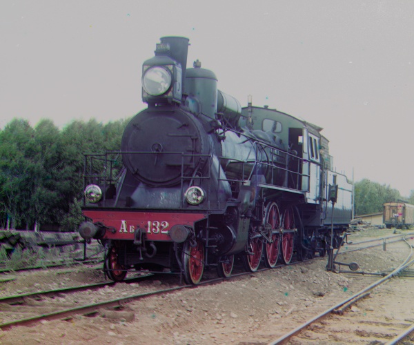
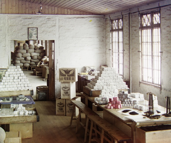
All the final results of the example images are shown below.
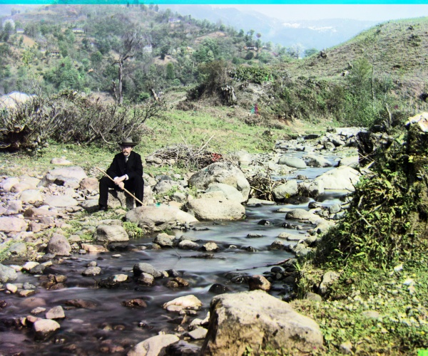
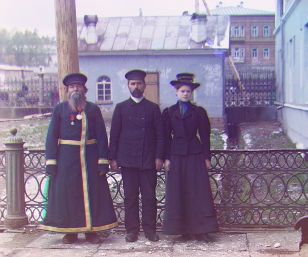
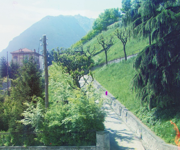
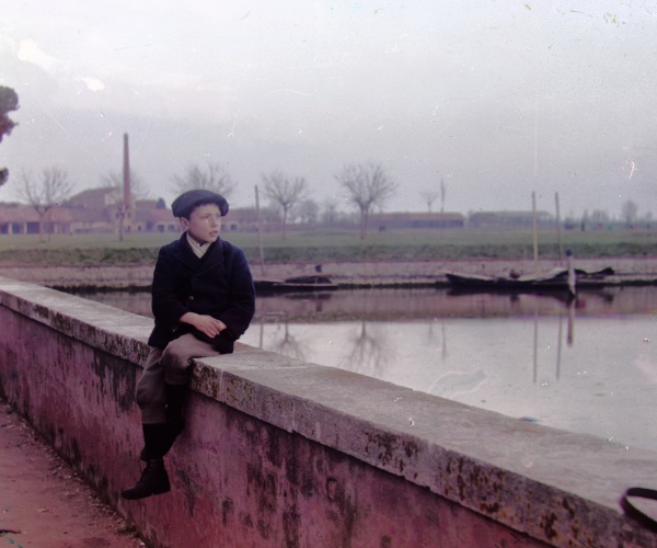
I have selected two extra images from the collection and the results are shown below.
| Name | displacement on the R channel | displacement on the G channel |
|---|---|---|
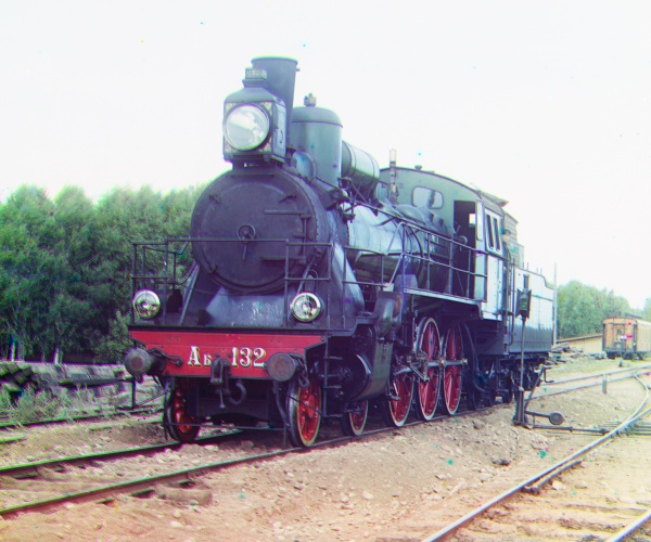
| train | (29, 85) | (6, 47) |
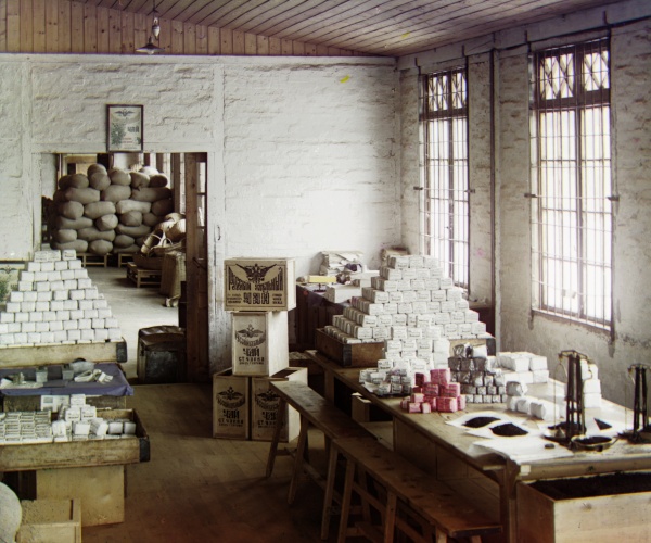
| workshop | (-12, 105) | (-1, 53) |
| melon | (14, 177) | (10, 80) |
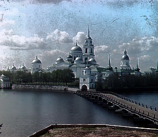
| monastery | (2, 3) | (2, -3) |
| lady | (13, 120) | (10, 56) |
| harvesters | (10, 124) | (17, 60> |
| icon | (22, 87) | (16, 39) |
| emir | (40, 107) | (23, 49) |
| castle | (4, 98) | (4, 36) |
| cathedral | (3, 12) | (2, 5) |
| tobolsk | (3, 6) | (3, 3) |
| self_portrait | (37, 175) | (29, 77) |
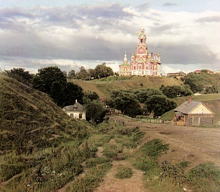
| onion_church | (34, 107) | (24, 52) |
| three_generations | (8, 112) | (12, 56) |