Project 1: Colorizing the Prokudin-Gorskii photo collection
Simona Aksman
Contents
- Overview
- Example JPEG images with blue channel alignment
- Example TIFF images with blue channel alignment
- Improving results for emir.tif: trying different base channels for alignment
- Additional selected images from collection with blue channel alignment
- Results of automatic contrasting and white balancing
Overview
The objective of this project was to take digitized Prokudin-Gorskii glass plate images, representing the red, green, and blue color channels, and write a program that could automatically produce a color image with as few visual artifacts as possible. We were given small JPEG images as well as larger TIFF images and asked to handle both use cases.
Most of my time was spent writing functions to align the channels. To align the low resolution JPEG images, I wrote a function called align() that aligns two color channels at a time by searching a [-15, 15] pixel window of potential x,y pixel offsets between the channels, and then finding the offset that maximizes the similarity between the channels. I used normalized cross-correlation (NCC) to find the similarity between channels after trying both Sum of Squared Differences distance and NCC. I found both of these metrics worked well but my implementation of NCC ran a bit faster, so I chose that one.
For the example JPEG images provided, I used align() with the blue color channel as the base channel, and this worked quite well. However, as expected, this function was too slow to use on the large TIFF images. I then wrote another function, recursive_align(), that makes use of the concept of "image pyramids" to recursively resize the two channels by a factor of 2, from coarse to fine, and then calculate offset values at each step. The function also upscales the offset values by a factor of 2 at each level and uses these offset values to narrow in on an offset selection. Since the example TIF files provided were about 10x the size of the example JPEGs, and I know that align() ran quickly for the JPEGs at that scale, I initialized the scaling factor for recursive_align() to 10. recursive_align() also uses NCC to make comparisons between channels, and the blue channel is used as the base for comparisons. Overall, this approach worked well on almost all of the high resolution images, except for emir.tif. I found that, for this image, using the green or red channel as my base worked much better than blue. I'm still not sure why this worked better, but I can see from the raw image that there seems to be a large difference in pixel intensity between red and blue (the colors on the man's jacket are inverted when comparing across these two channels), and perhaps this dissimilarity in color channels made it harder to align when the blue channel was the base.
Overall, since blue channel alignment worked well for most images, I used that for the rest of the example TIFF images as well as some additional images from the Prokudin-Gorskii collection.
Cropping
I cropped all channels by 10% on all sides before alignment, which helped to reduce some of the alignment issues I experienced in early iterations of the program. After alignment, I cropped by 1% on both sides, and 5% on the top and bottom of each image. This helped to further reduce some of the residual artifacts left from the alignment process.Automatic contrasting
Some of the color images (such as mill_near_luga.tif) initally had poor contrast and therefore appeared washed out, so I tried Histogram Equalization, which maps the image's pixel intensity distribution to its cumulative distribution function. This has the effect of making the pixel intensity of the image more uniform. In my program, this operation is applied to the raw image before splitting the color channels. Across all of the images tested, applying this transformation seemed to improve the visibility of granualar details in parts of the image that appeared washed out.Automatic white balancing
I also applied automatic white balancing by finding the brightest pixel value for each of the color channels, and then finding the brightest value across the three channels. I applied a Gaussian blur before picking the brightest pixel because this is supposed to make the pixel selection process less susceptible to noise. This value was then used as my illuminant (expected source of visible light). I scaled each color channel to match the brightness of the illuminant. In general, white balancing seems to have improved most of the images, with the exception of workshop.tif. The impact of this step appears to be most visible in places where the pixels are at their highest intensity, such as in the sky of train.tif or monastery.jpeg. It may have had less of an impact on workshop.tif because that photo was taken indoors.If I had more time, I would try optimizing the kernel size (radius) of the Gaussian blur more. I came up with a somewhat arbitrary rule for setting the kernel size:
2 * int(np.log2(channel.shape[1])) - 1. I set it this way because I wanted the kernel to be much smaller than the image, and also it needed to be an odd number (as this is a requirement of the cv2.GaussianBlur() function).
Example JPEG images with blue channel alignment
Offsets provided below each image.
cathedral.jpeg
green: [5, 2]
red: [12, 3]
tobolsk.jpeg
green: [3, 3]
red: [6, 3]
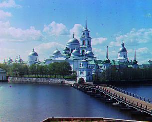
monastery.jpeg
green: [-3, 2]
red: [3, 2]
Example TIFF images with blue channel alignment
lady.tif
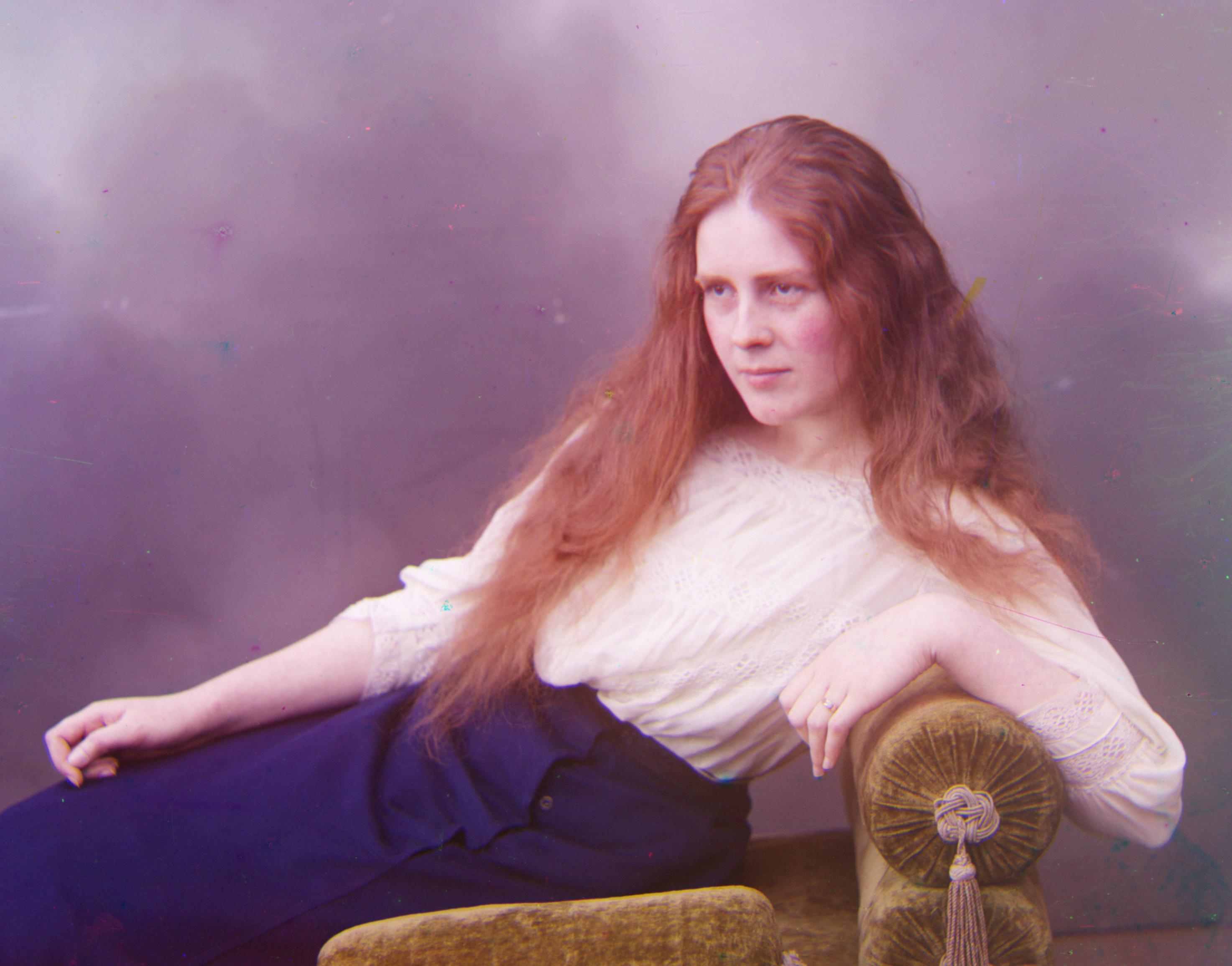
green: [50, 8]
red: [112, 12]
melons.tif
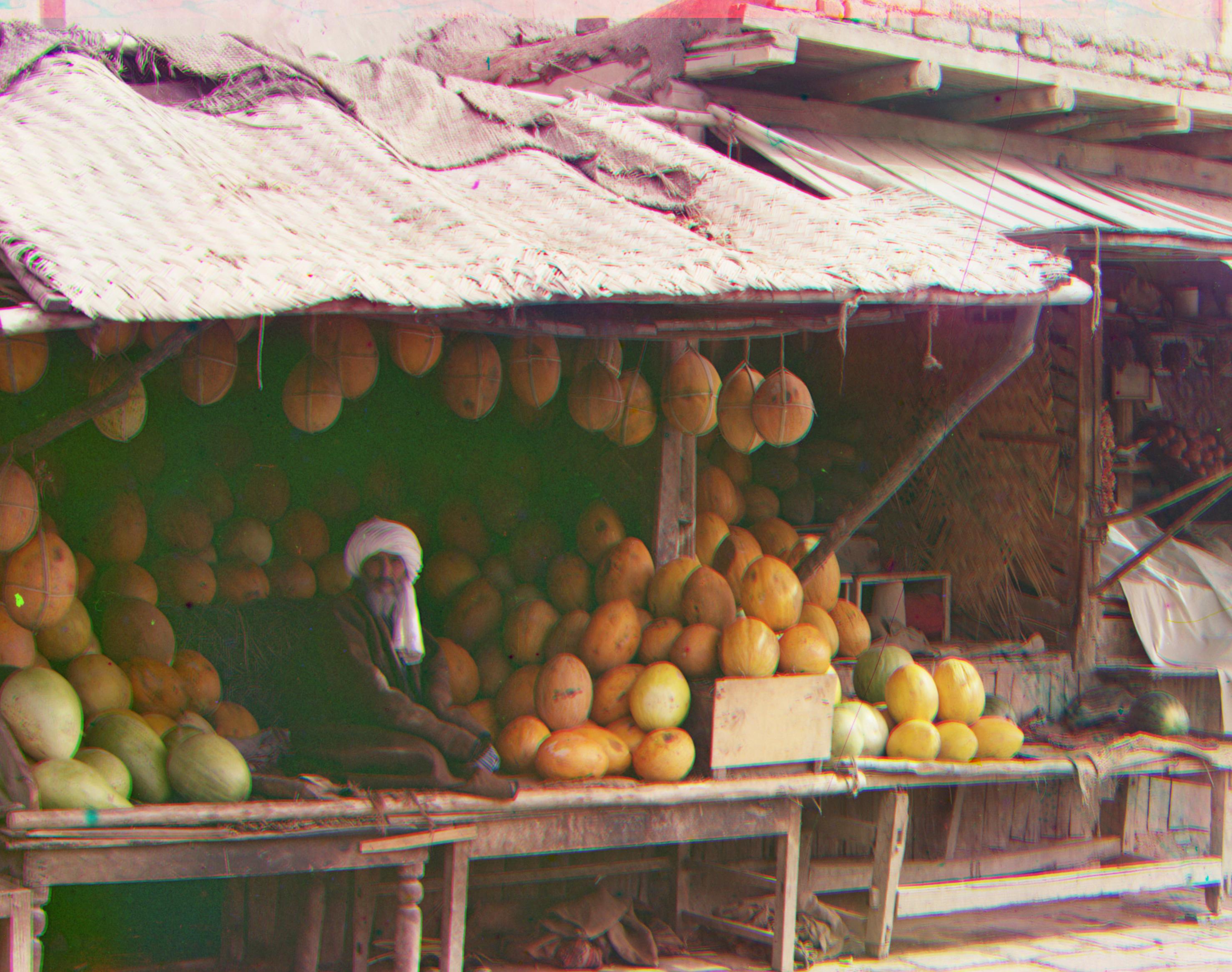
green: [82, 10]
red: [172, 10]
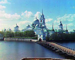
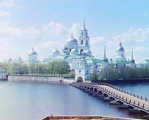
onion_church.tif
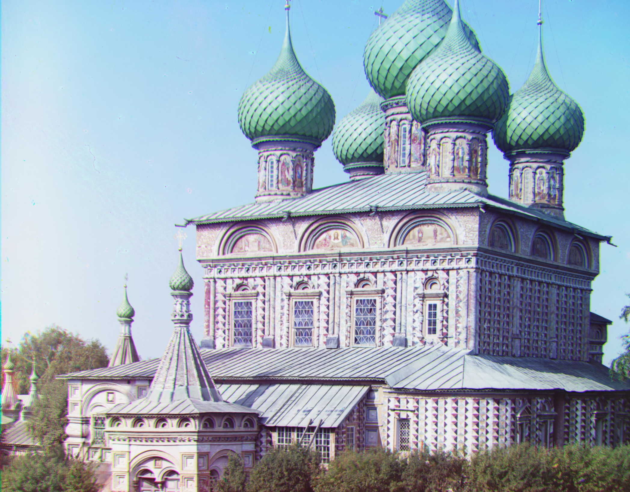
green: [52, 26]
red: [108, 36]
self_portrait.tif
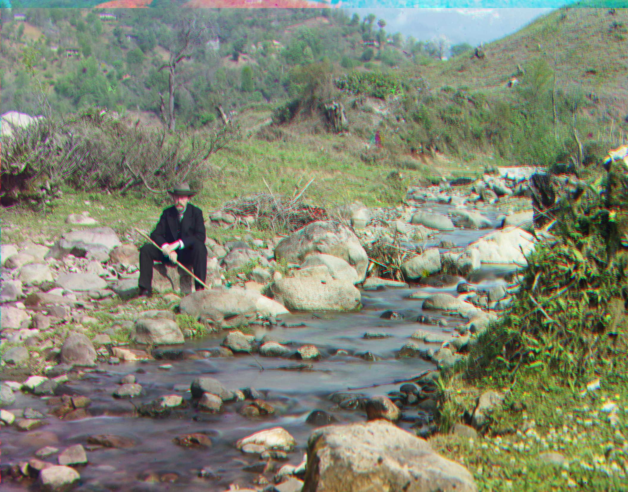
green: [78, 28]
red: [168, 34]
three_generations.tif
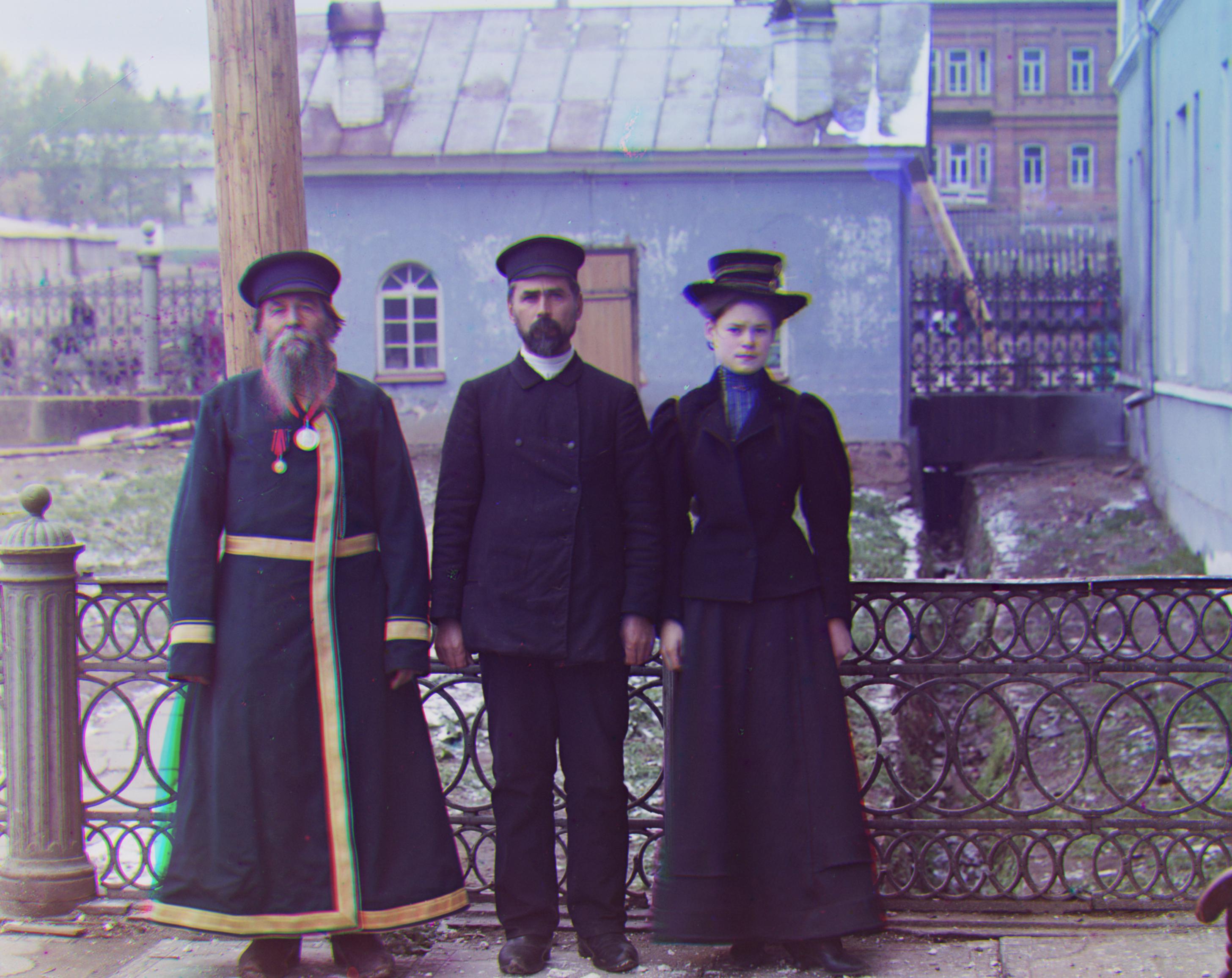
green: [54, 14]
red: [112, 10]
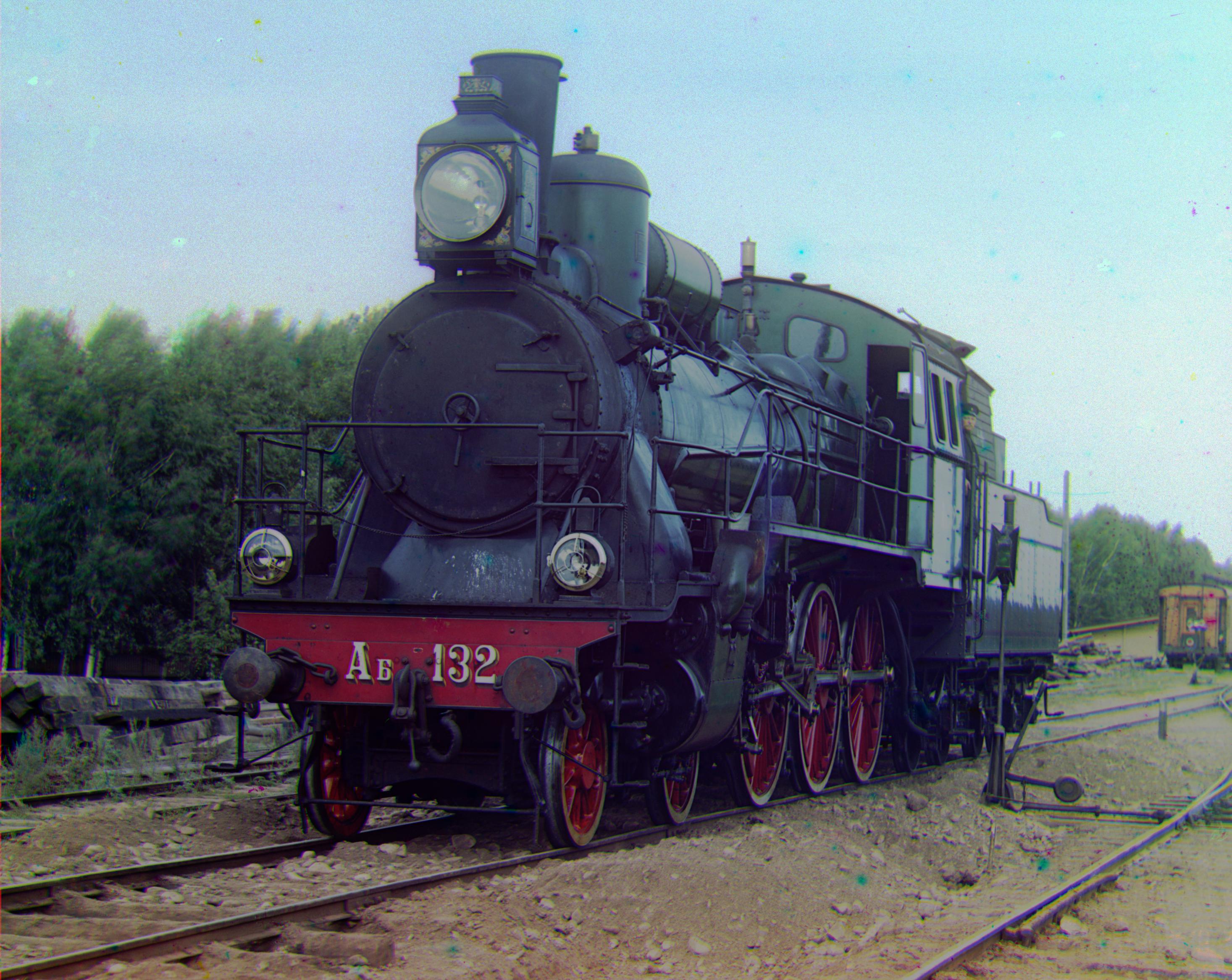
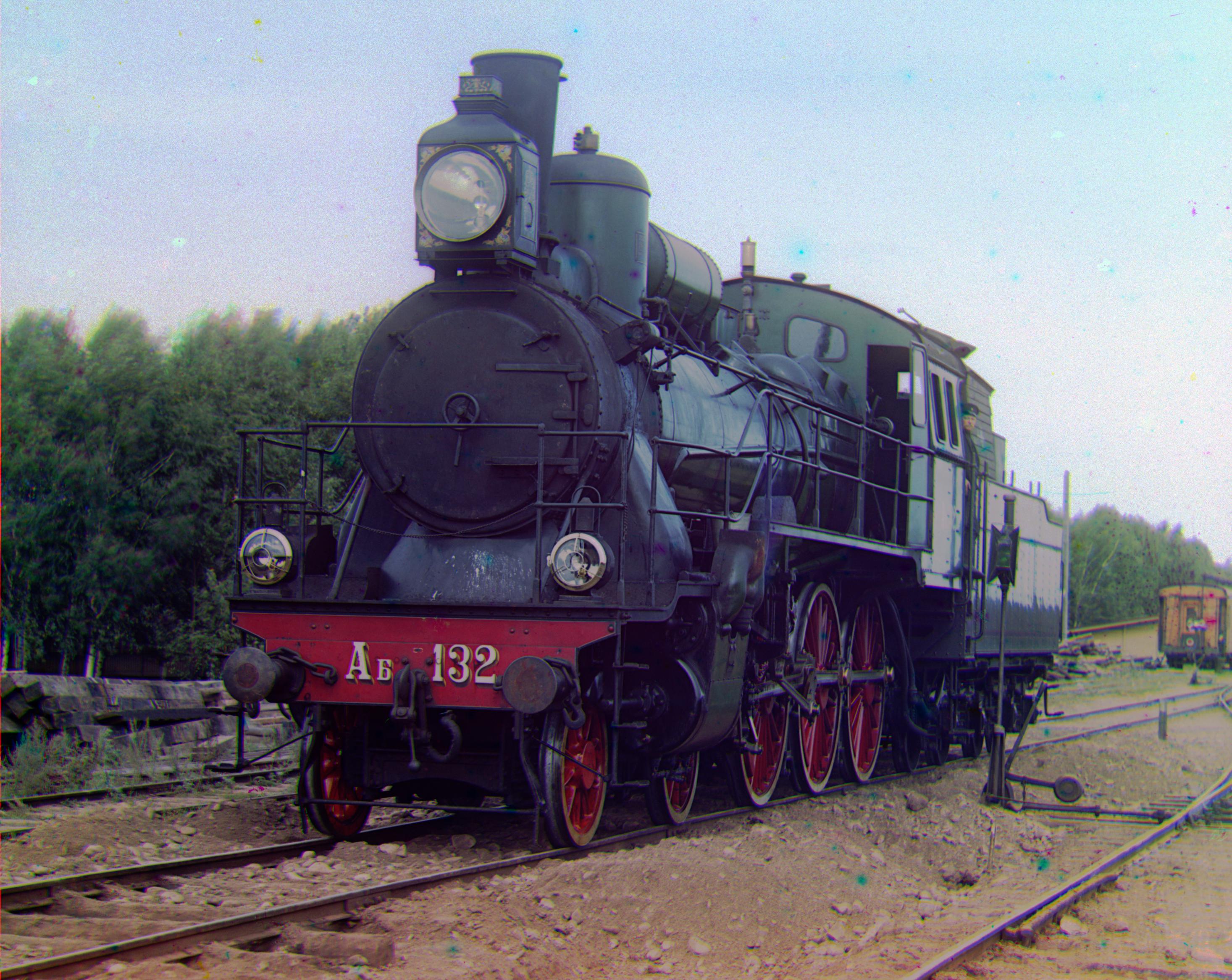
train.tif
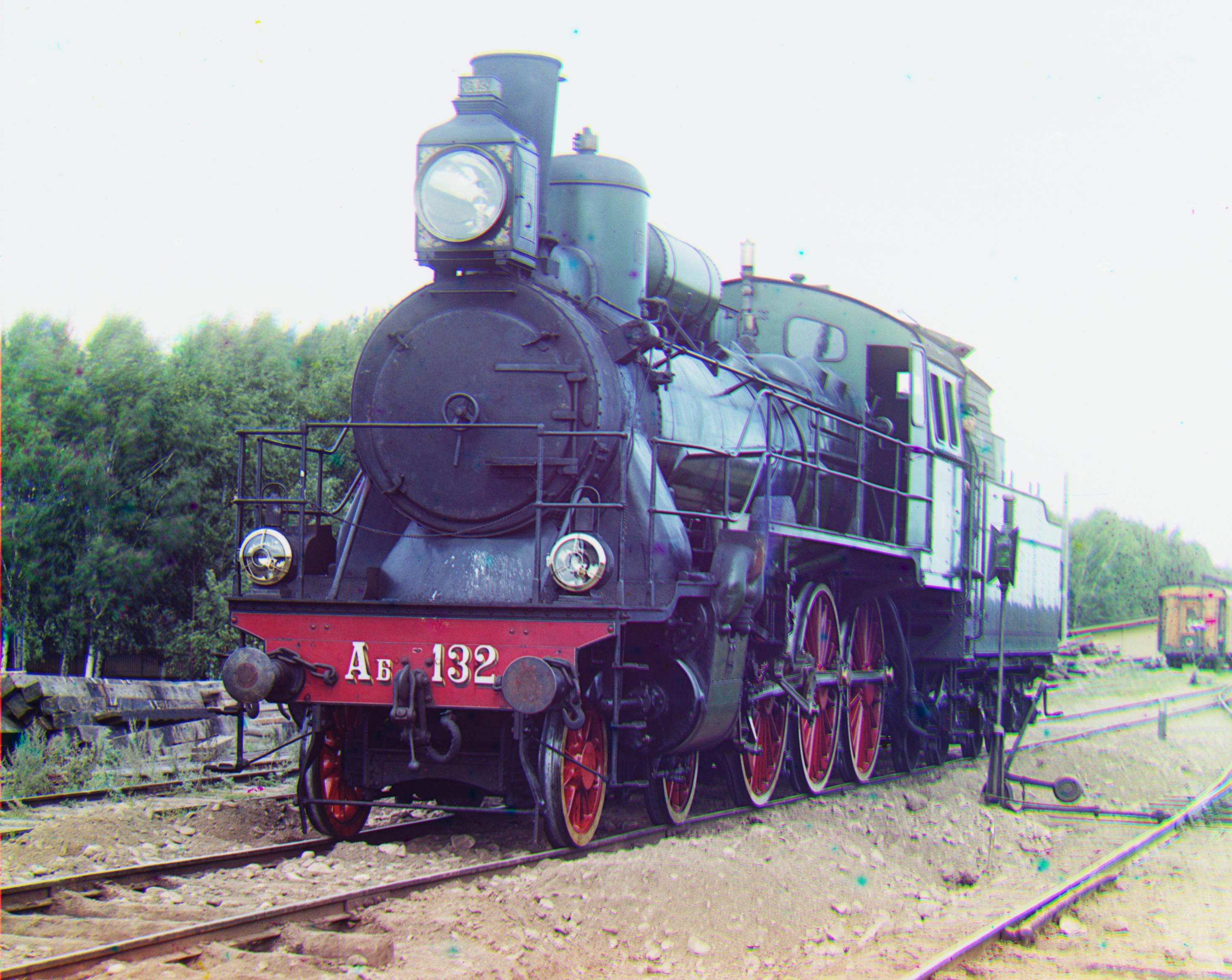
green: [42, 4]
red: [88, 32]
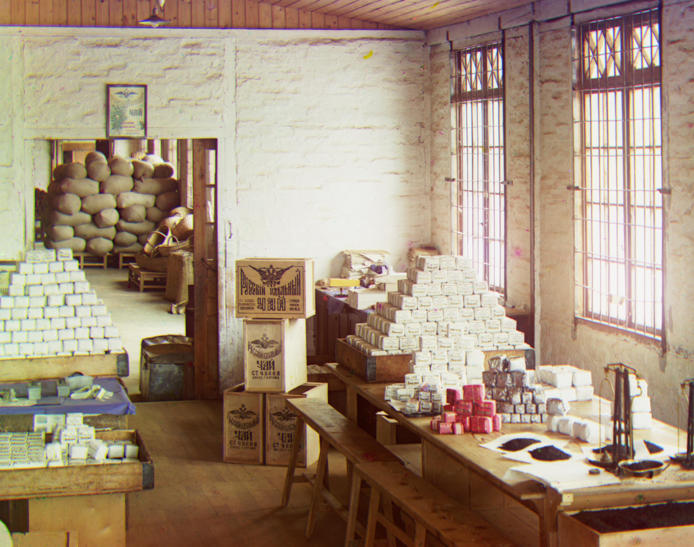
workshop.tif
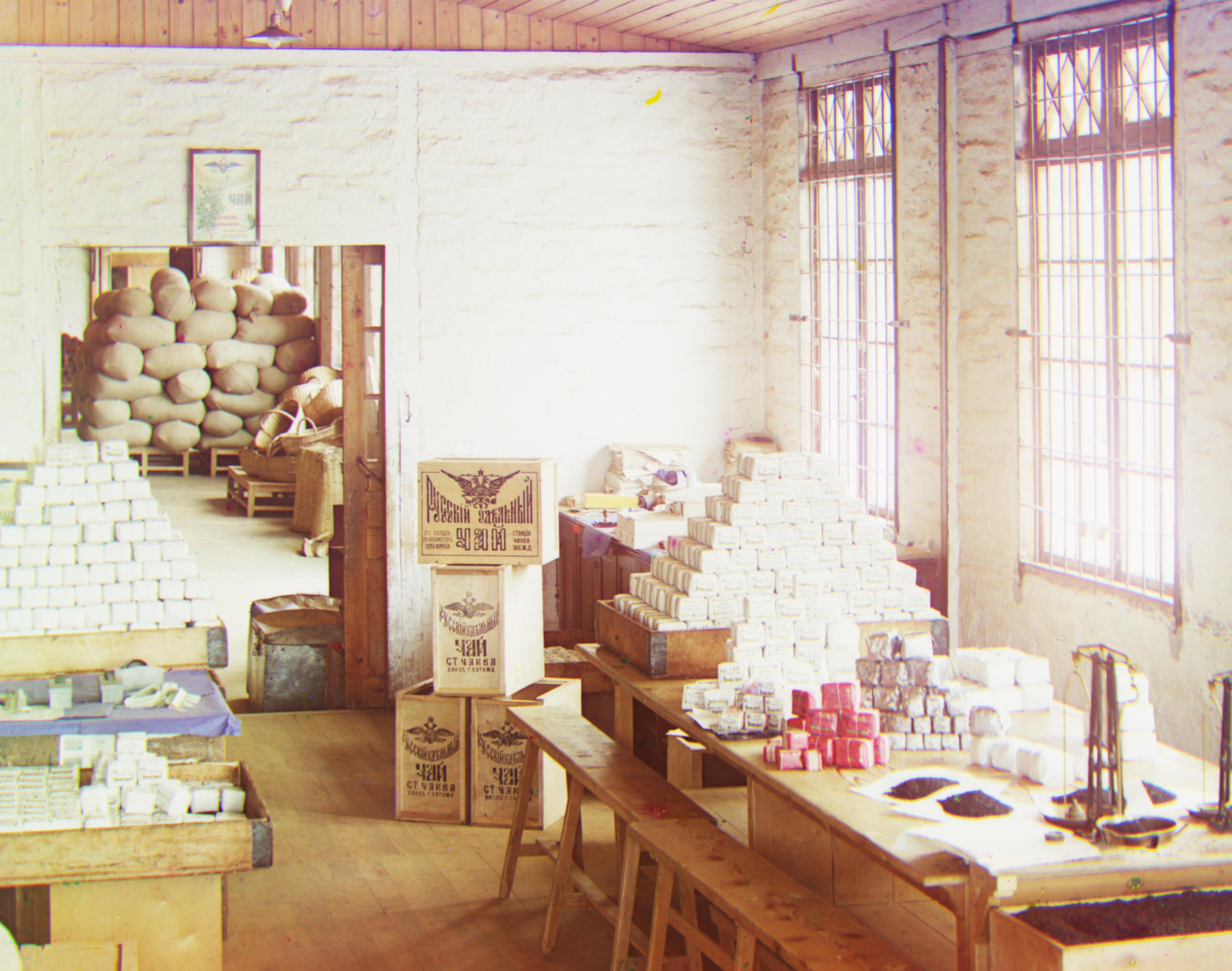
green: [52, 0]
red: [104, -12]
harvesters.tif
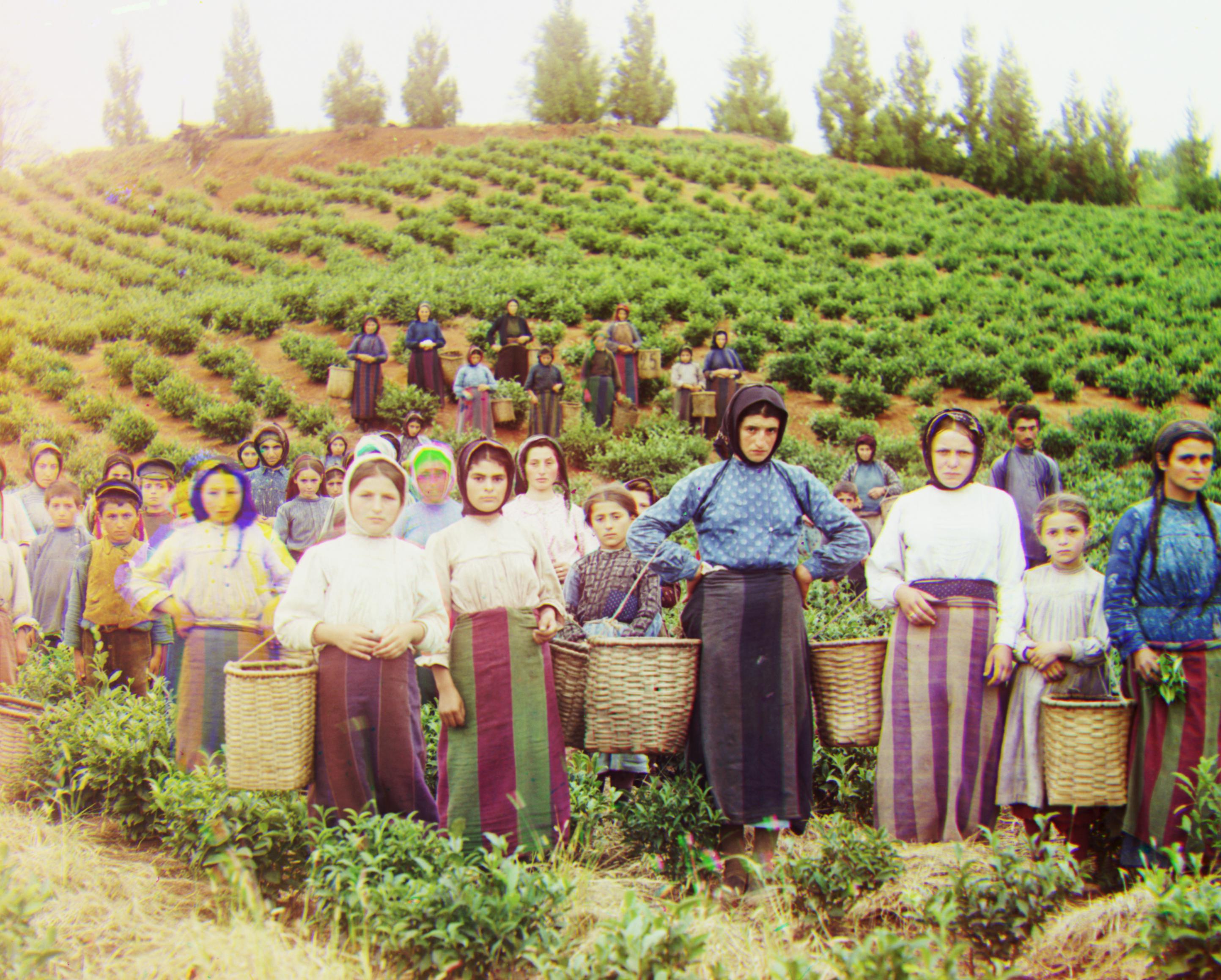
green: [60, 16]
red: [124, 14]
icon.tif
green: [40, 16]
red: [90, 22]
church.tif
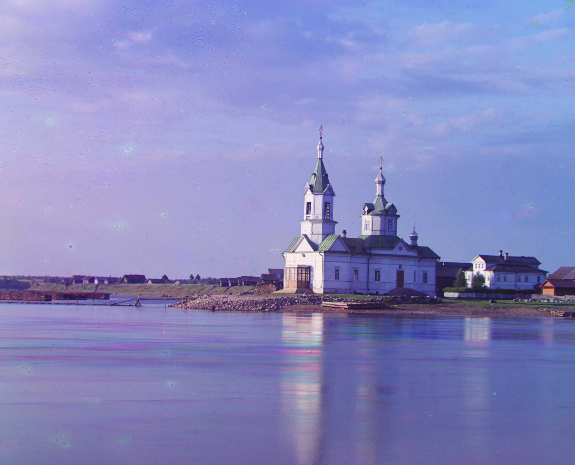
green: [24, 4]
red: [58, -4]
emir.tif
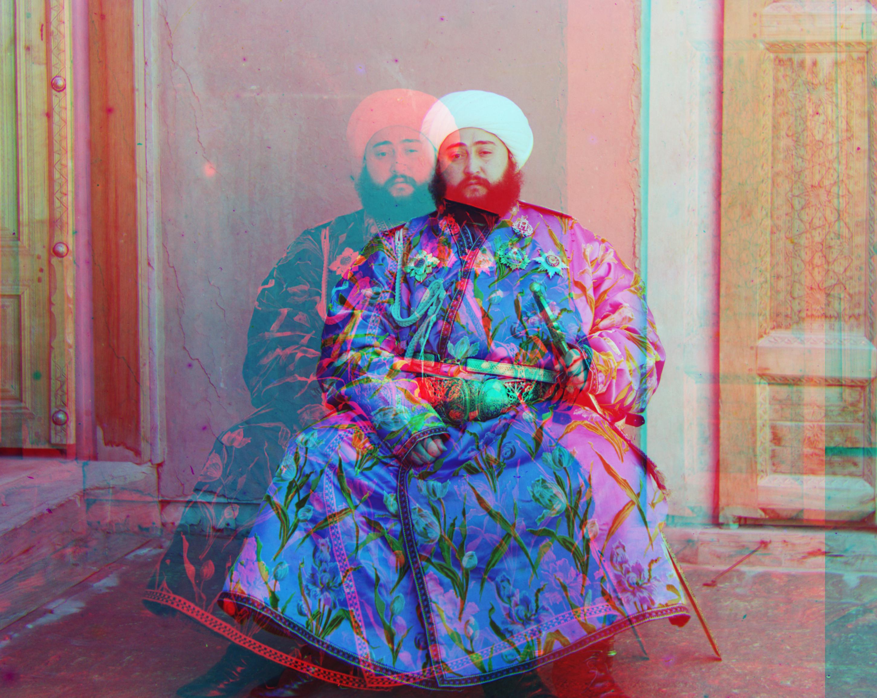
green: [48, 24]
red: [100, -202]
Improving results for emir.tif: trying different base channels for alignment
red
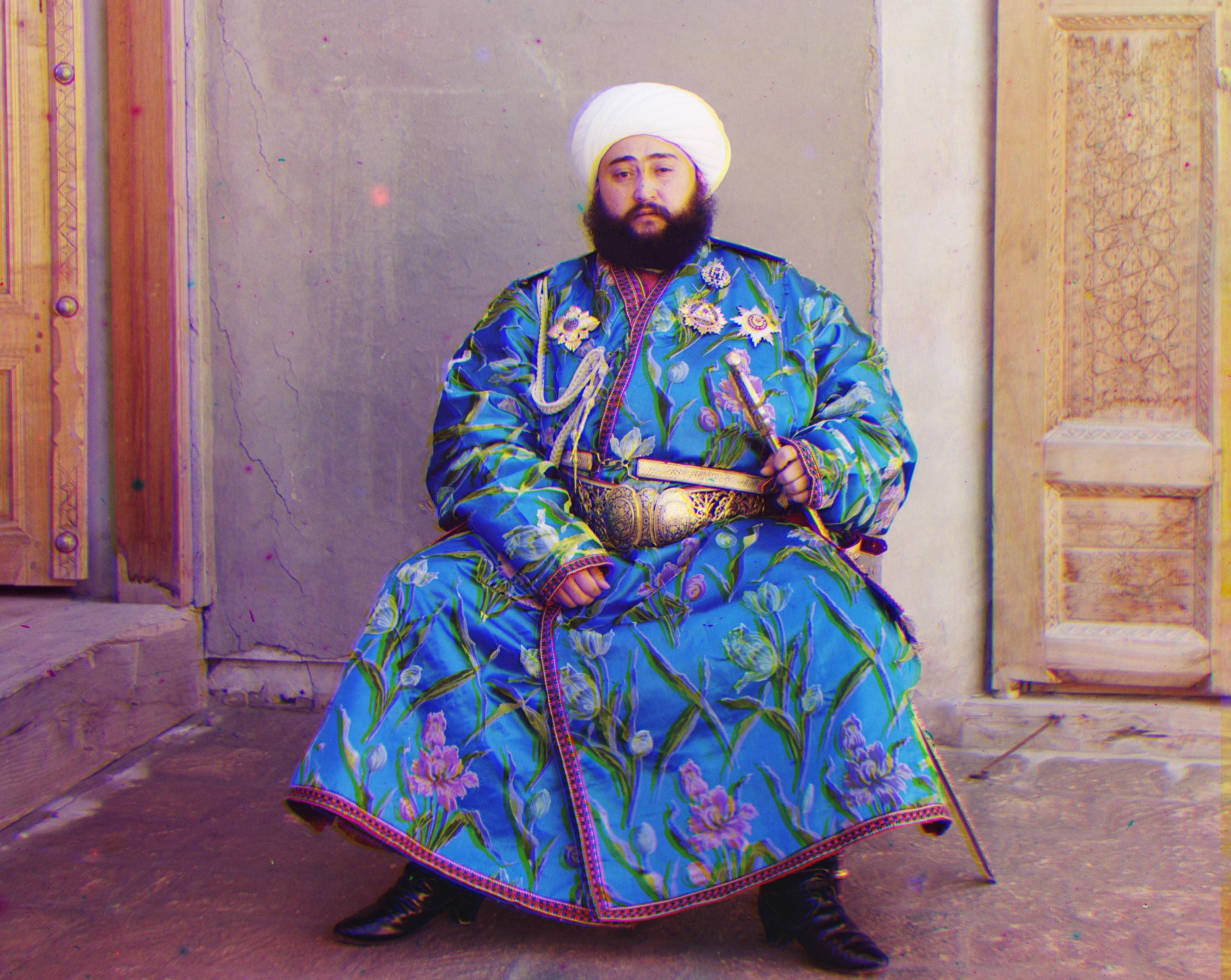
green: [-56, -18]
blue: [-102, -54]
green
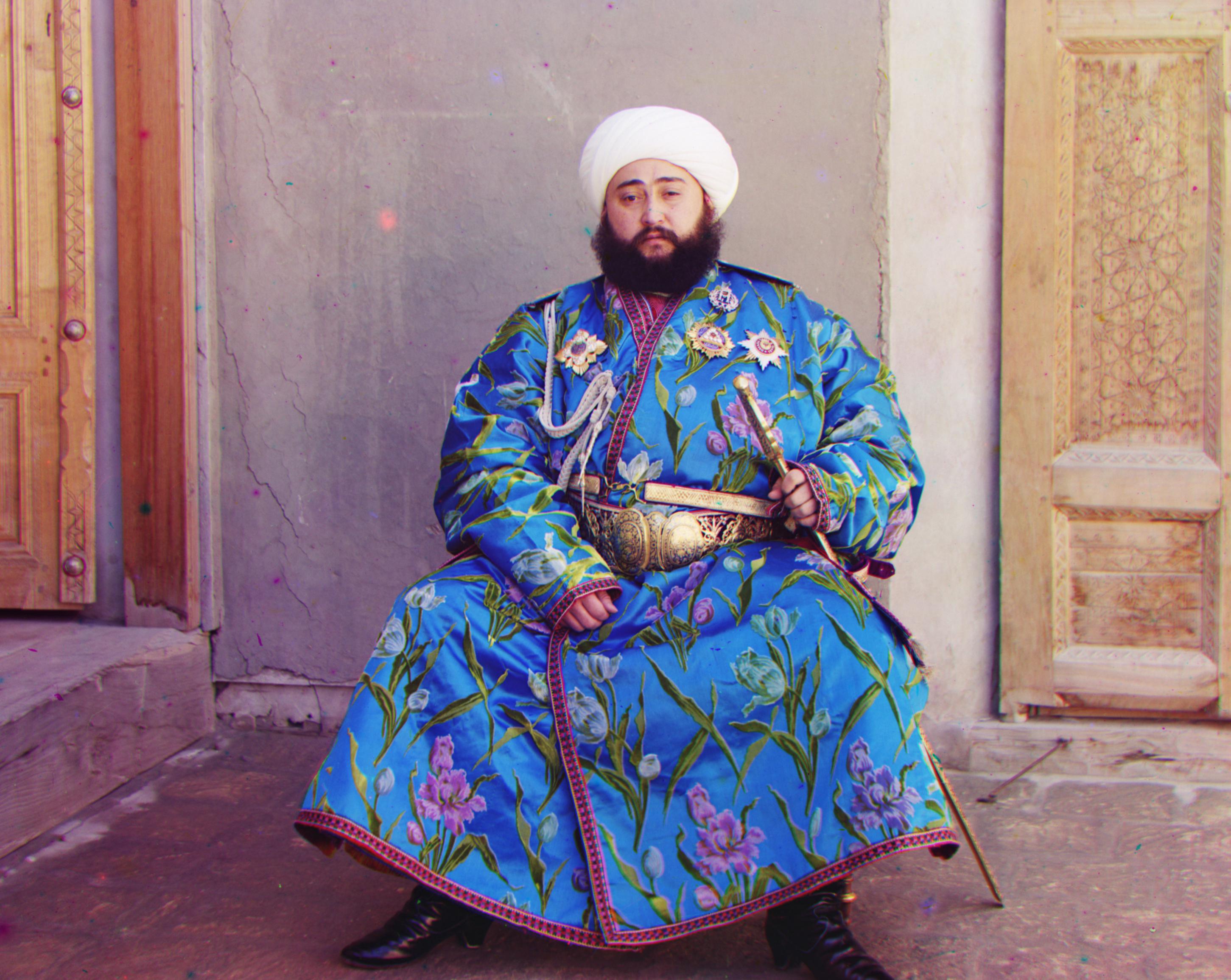
blue: [-48, -24]
red: [56, 18]
blue
green: [48, 24]
red: [100, -202]
Additional selected images from collection with blue channel alignment
peasant_girls.tif
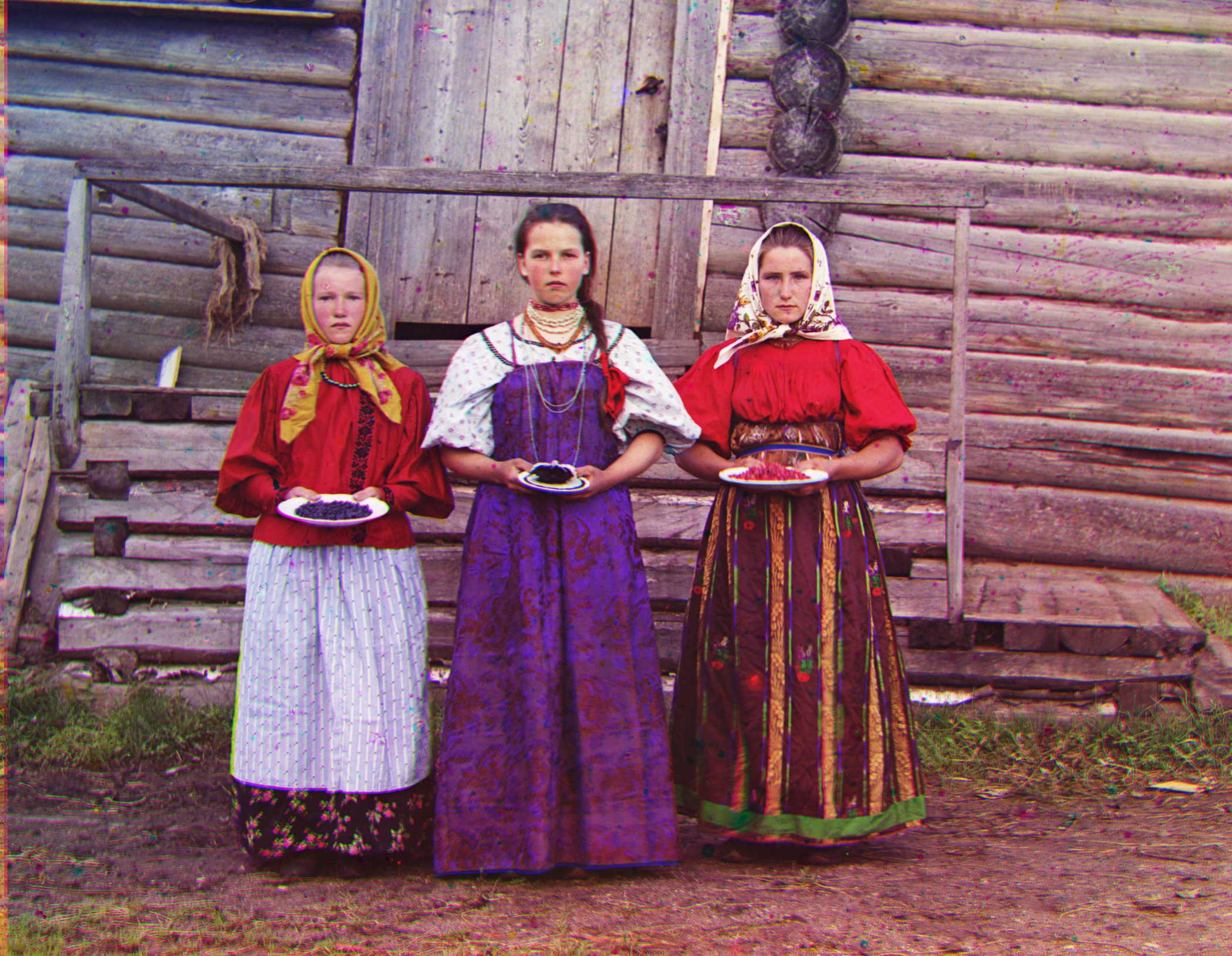
green: [-16, 10]
red: [10, 18]
cornflowers_in_field_of_rye.tif

green: [14, 6]
red: [40, 0]
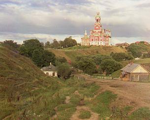
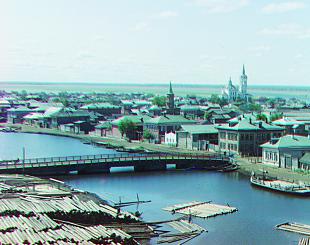
mill_near_luga.tif
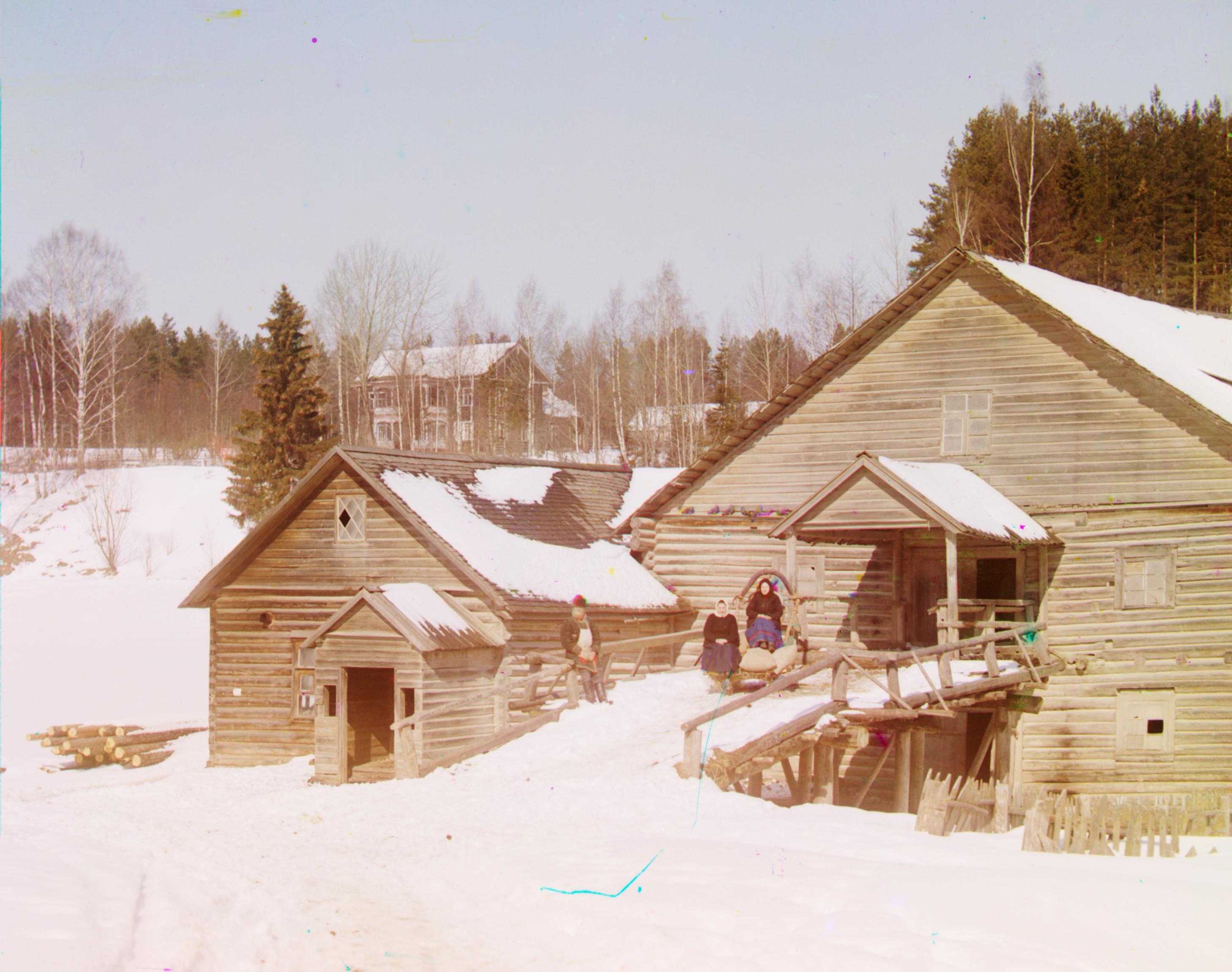
green: [10, 16]
red: [90, 32]
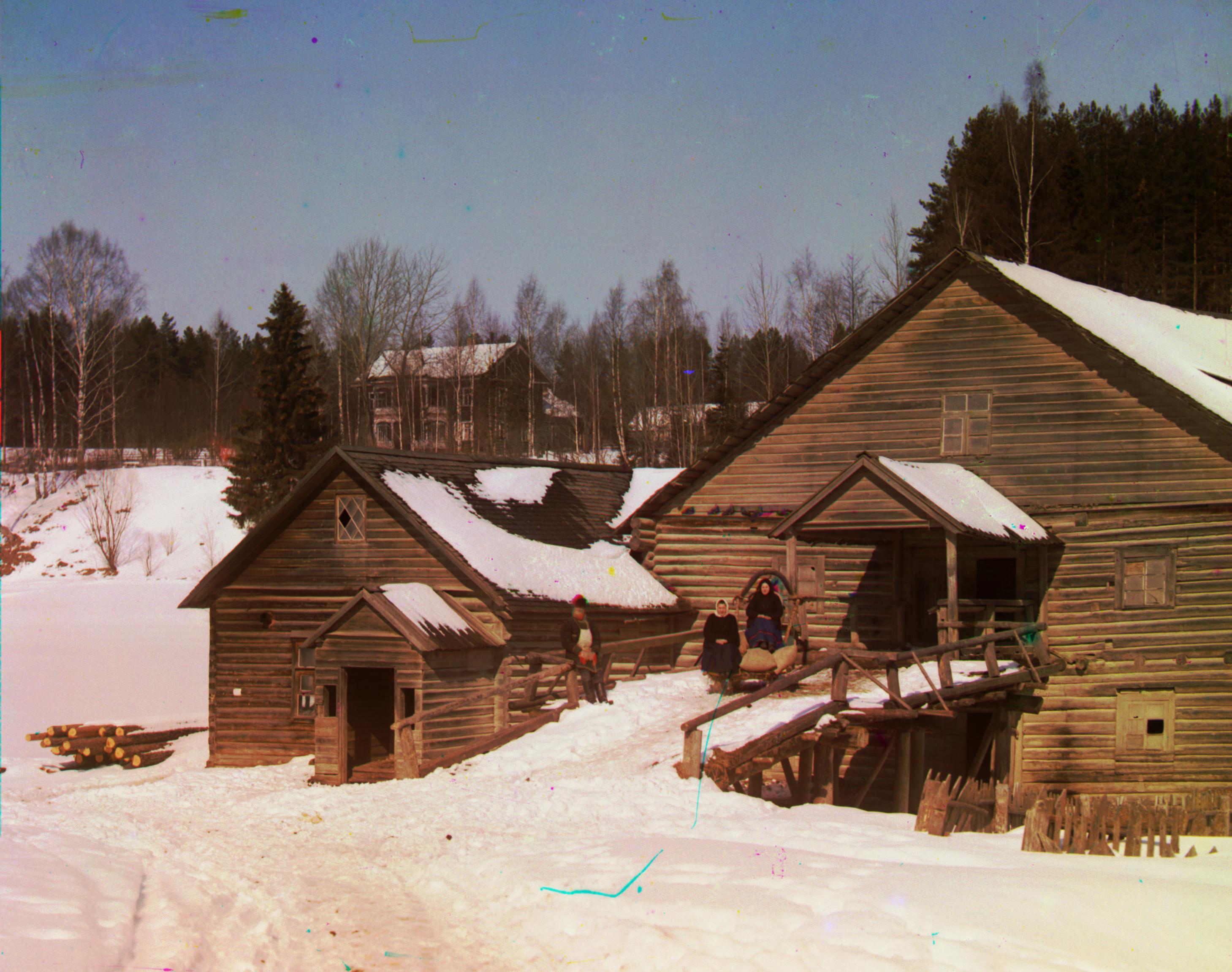
Results of automatic contrasting and white balancing
before
after, contrasting only
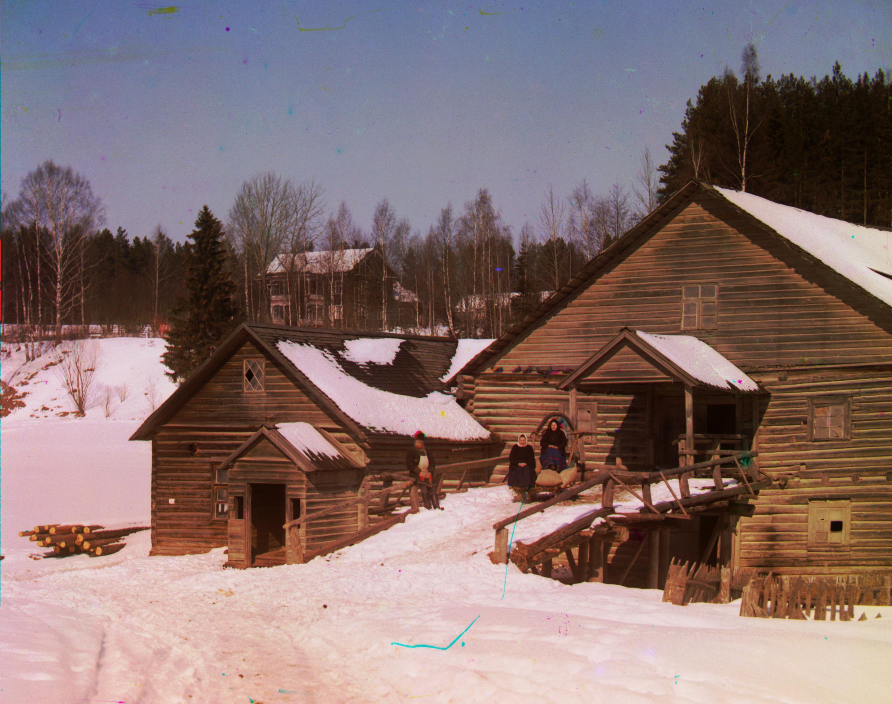
after, contrasting + white balancing
before
after, contrasting only
after, contrasting + white balancing
before
after, contrasting only
after, contrasting + white balancing

before
after, contrasting only
after, contrasting + white balancing