Colorizing the Prokudin-Gorskii Photo Collection

In 1907, Sergei Mikhailovich Prokudin-Gorskii travelled across the vast Russian Empire and take color photographs of everything he saw. However, at the time, there was no way to print color photographs. However, preparing for the future, Sergei recorded three exposures of every scene onto a glass plate using a red, a green, and a blue filter. Years later, these plates are still preserved. Recently, the Library of Congress combined these plates to produce these color images that Sergei was never able to see. In this project, I explored various methods for reconstructing these color images.

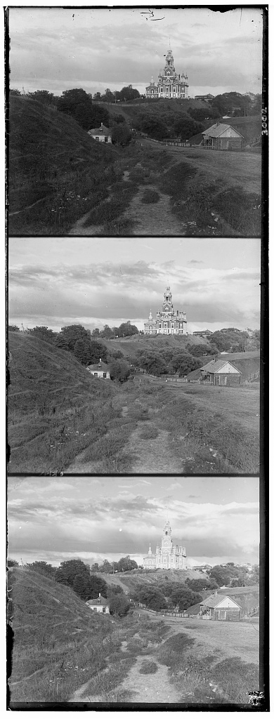
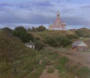
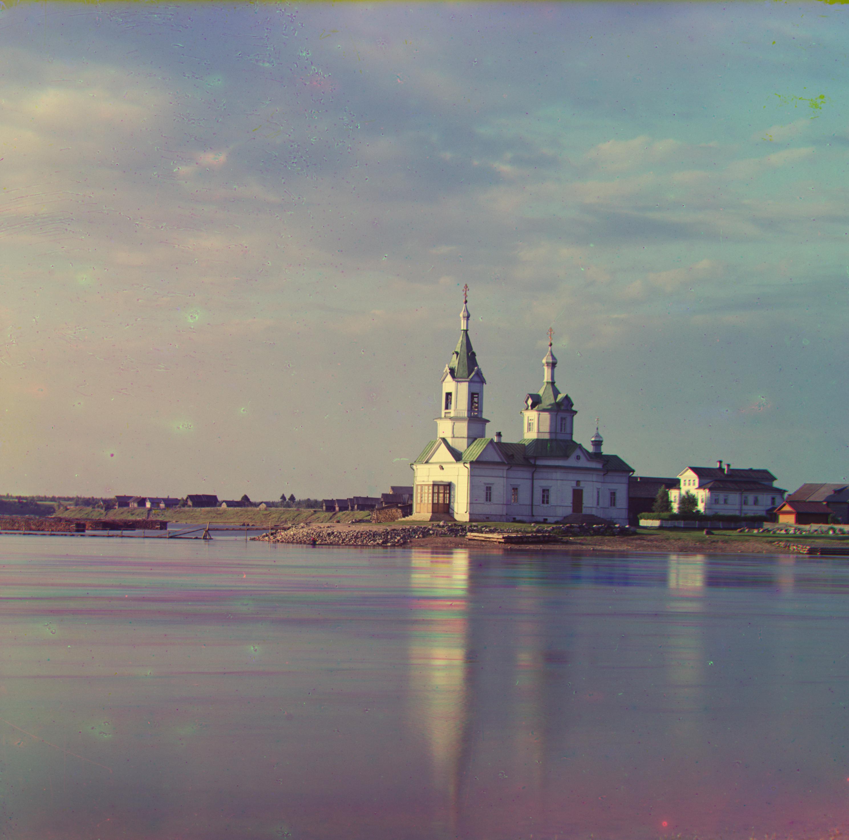
Here is a quick sample of the original color plates and the final reconstructed color image:

Simple Alignment

Aligning the negative filters to produce the colored image isn’t as easy as simply stacking the filters on top of each other. This is because each plate captured slightly different parts of the scene. So, the plates are shifted versions of the same image. If you simply aligned them on top of each other directly, you would get very noticable colored shadows demonstrating how the plates were unaligned.

To solve, I simply shifted both the green and red plates against the blue plate and calculated an offset that produced the best alignment. It is a very simple idea, but there is more to unpack. What exactly does “best” mean? We need some type of measurement function to see how well-aligned two images are. I approached this by using the sum of squared differences between two color plates. It is likely that a single image will have similar color intensities on each channel in the same spots, so finding the alignment that minimizes this difference would be an effective heurstic to solve this problem.

I used a window of size 8 along both axes to search for the best alignment. However, since there tends to be a lot of variability around the borders, I only make comparisons using the inner 60% of the image. We do get some decent results.

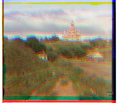
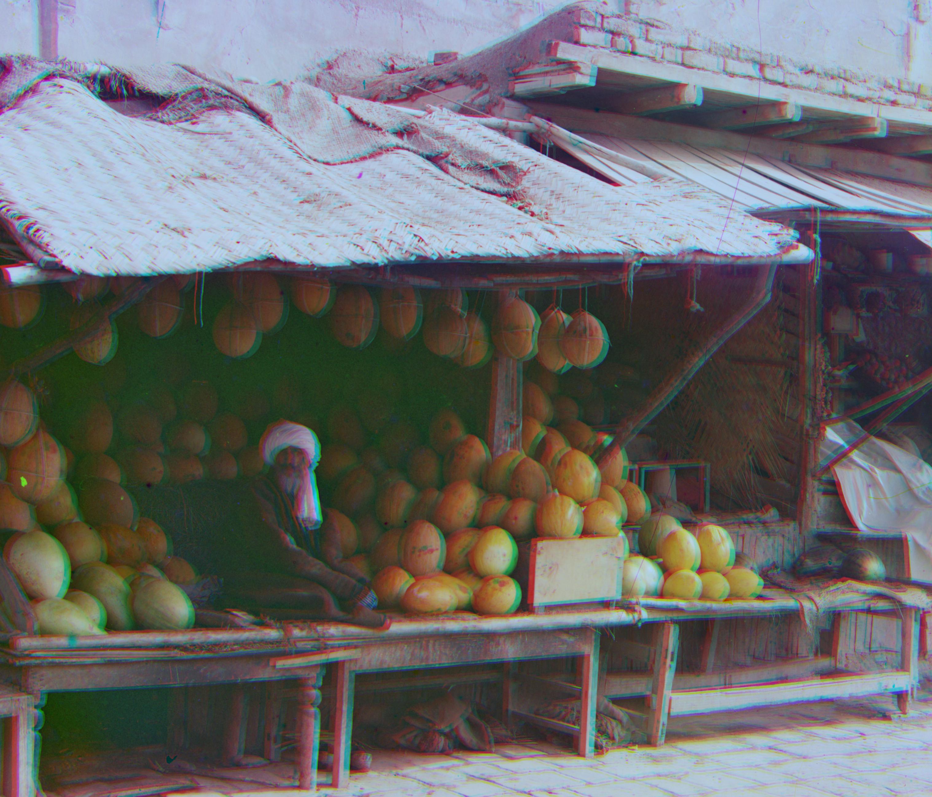
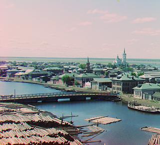
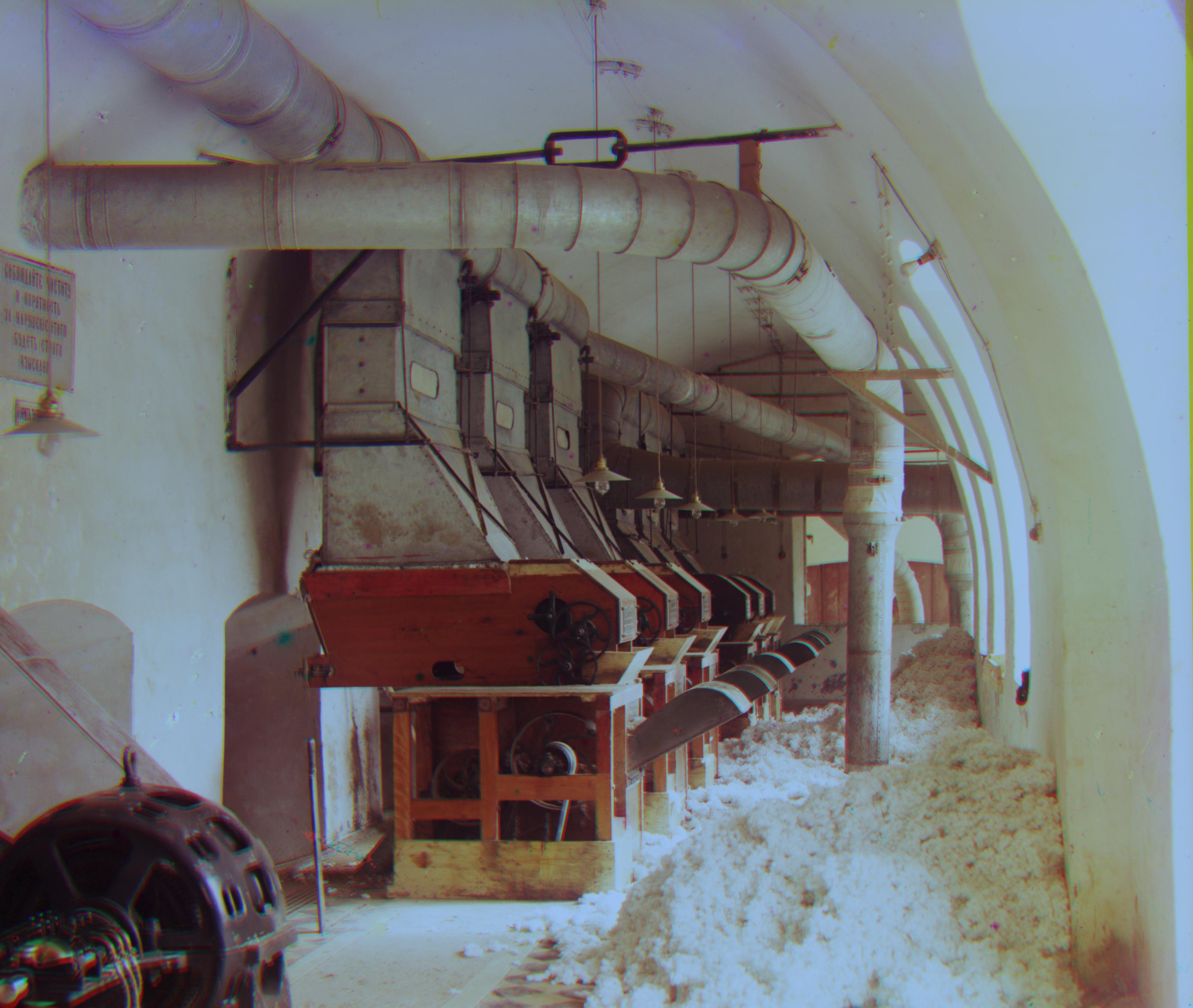
However, this wasn’t a magic solution that worked perfectly for all of the inputs. Let’s take a look at the following image:

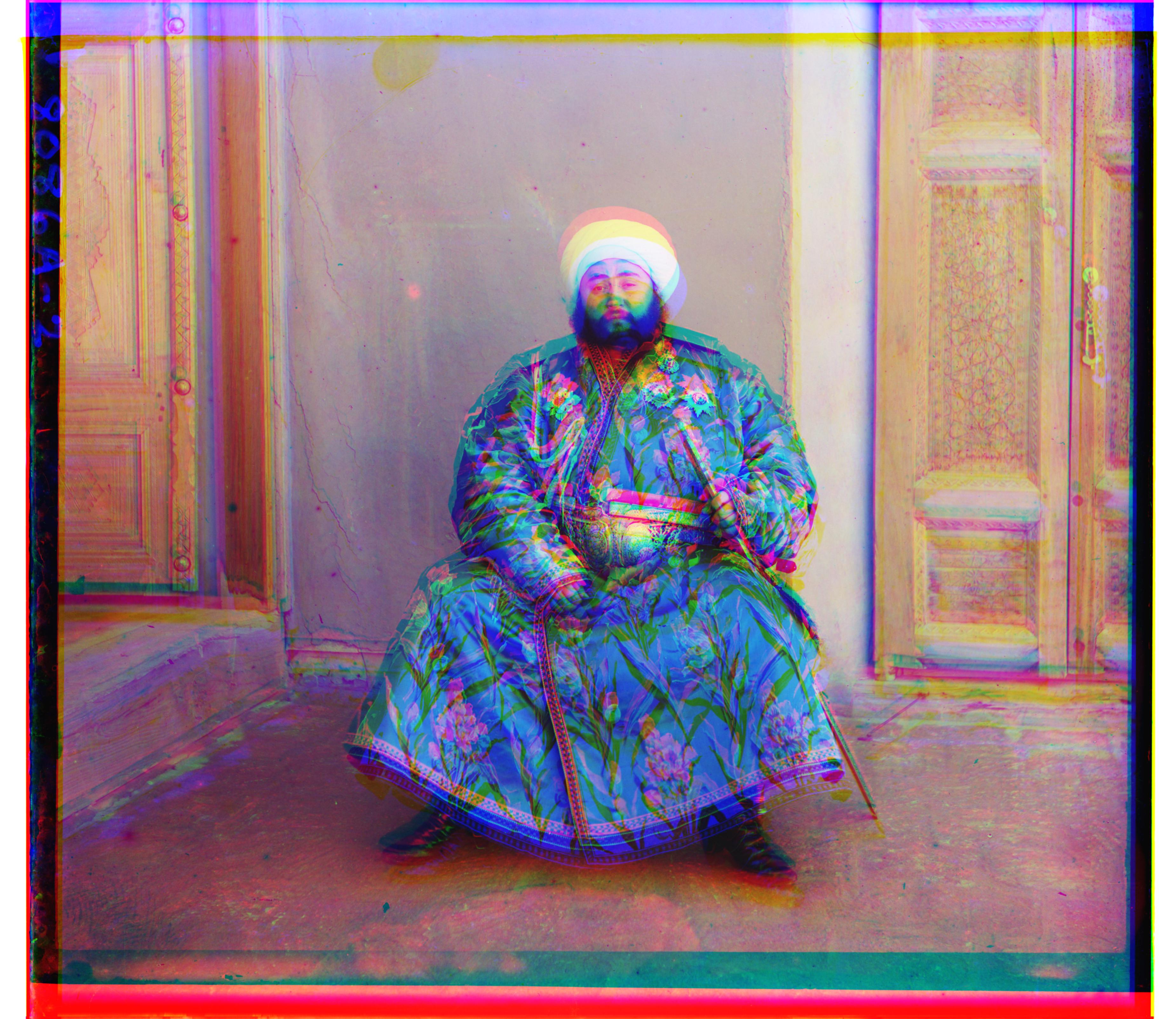
Notice there is still a lot of discoloration and this shadowing effect. The different color channels are bright at different locations so the alignment isn’t measuring exactly what we wanted. We need to find a better heuristic to match our color plates together.

Pyramid Alignment

Before, I dive into the other heuristics I used for solving the alignment problem, there is one other issue with the naive approach I described above. Mainly, it is simply too slow. Some of the images are several thousand by several thousand pixels big, so doing a large search plus an expensive alignment calculation isn’t very feasible. We need a faster approach. So, I employed the image pyramid technique. This enables us to localize our search by first aligning downscaled versions of each image and then using information from the smaller scale alignment to more precisely search for the best alignment at higher resolutions. This allows us to do very few comparisons at the full image resolution, while still being able to recreate and even improve on the results of the naive method.

In my implementation, I used 4 layers in my pyramid and scaled each layer by a factor of 2. I also set a window of size 2 to search around on the highest resolution image. This window scales in size as you decrease the resolution, which we can afford since the smaller images require less computation for scoring.

*Edge Detection

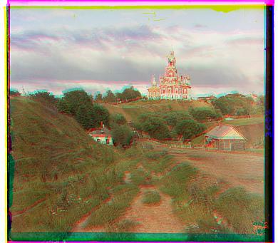
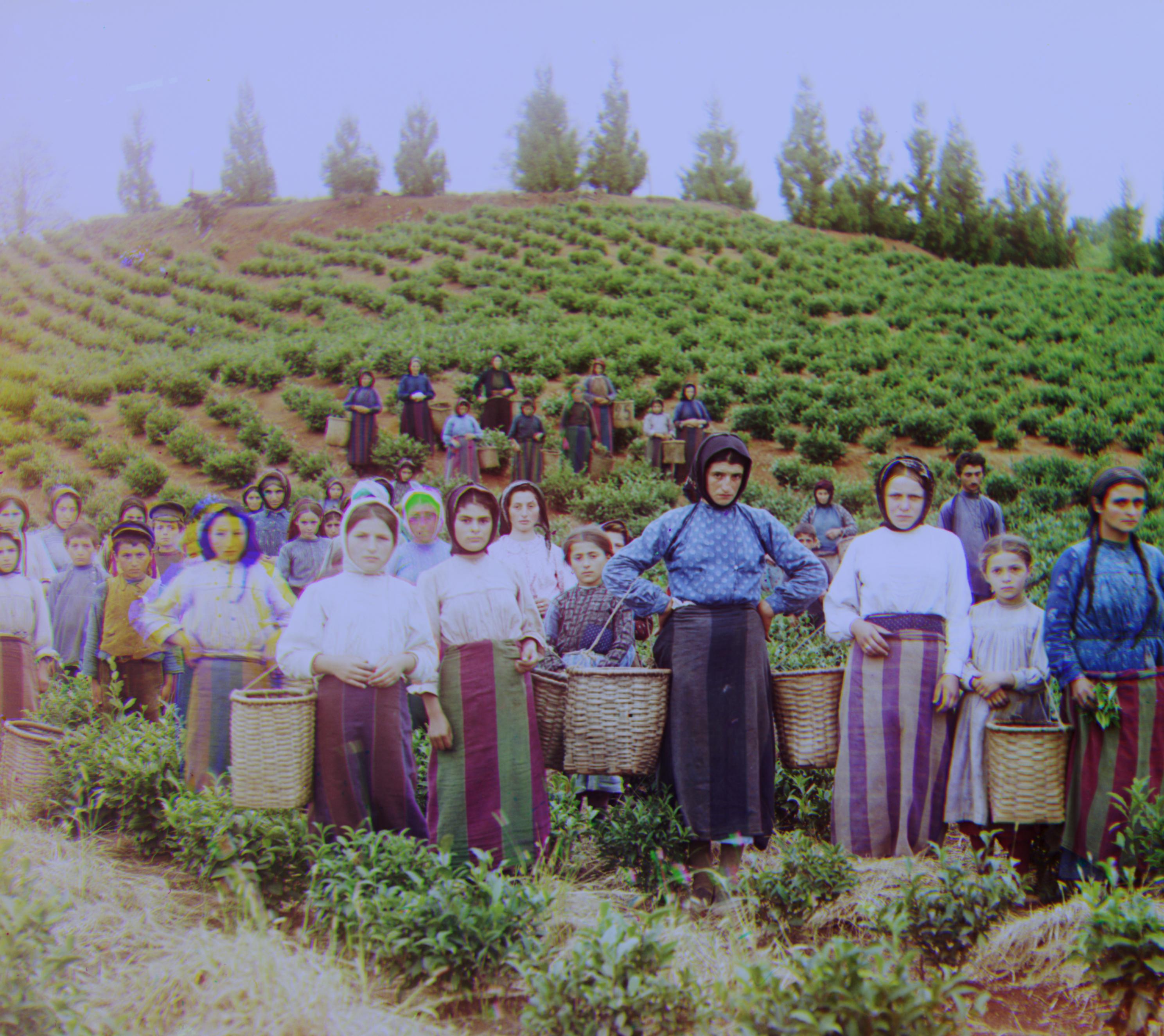
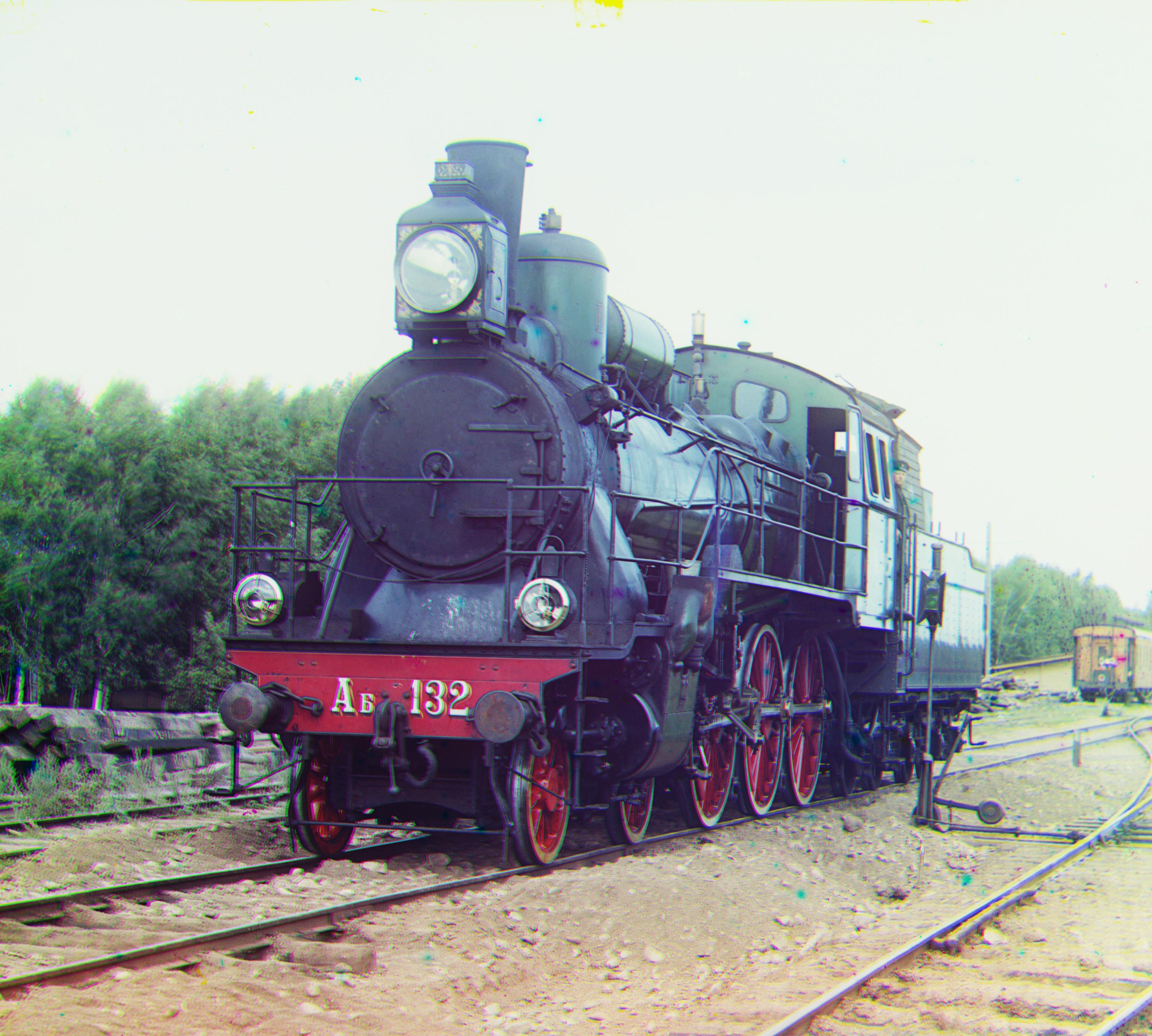
Now that we have an efficient algorithm for comparing larger images, we return back to the alignment problem. The issue is that using simply the pixel intensities as features for alignment is not good enough. We need something a bit more rich and consistent across each channel. So, I looked into seeing if the edges present in each of the channels would be a better alternative. I used the opencv Canny edge detection method to find all of the edges in each channel. Then, I aligned these edge maps using the image pyramid method and applied the found offset to the original color plate. This resulted in significant improvement. Let’s take a look:

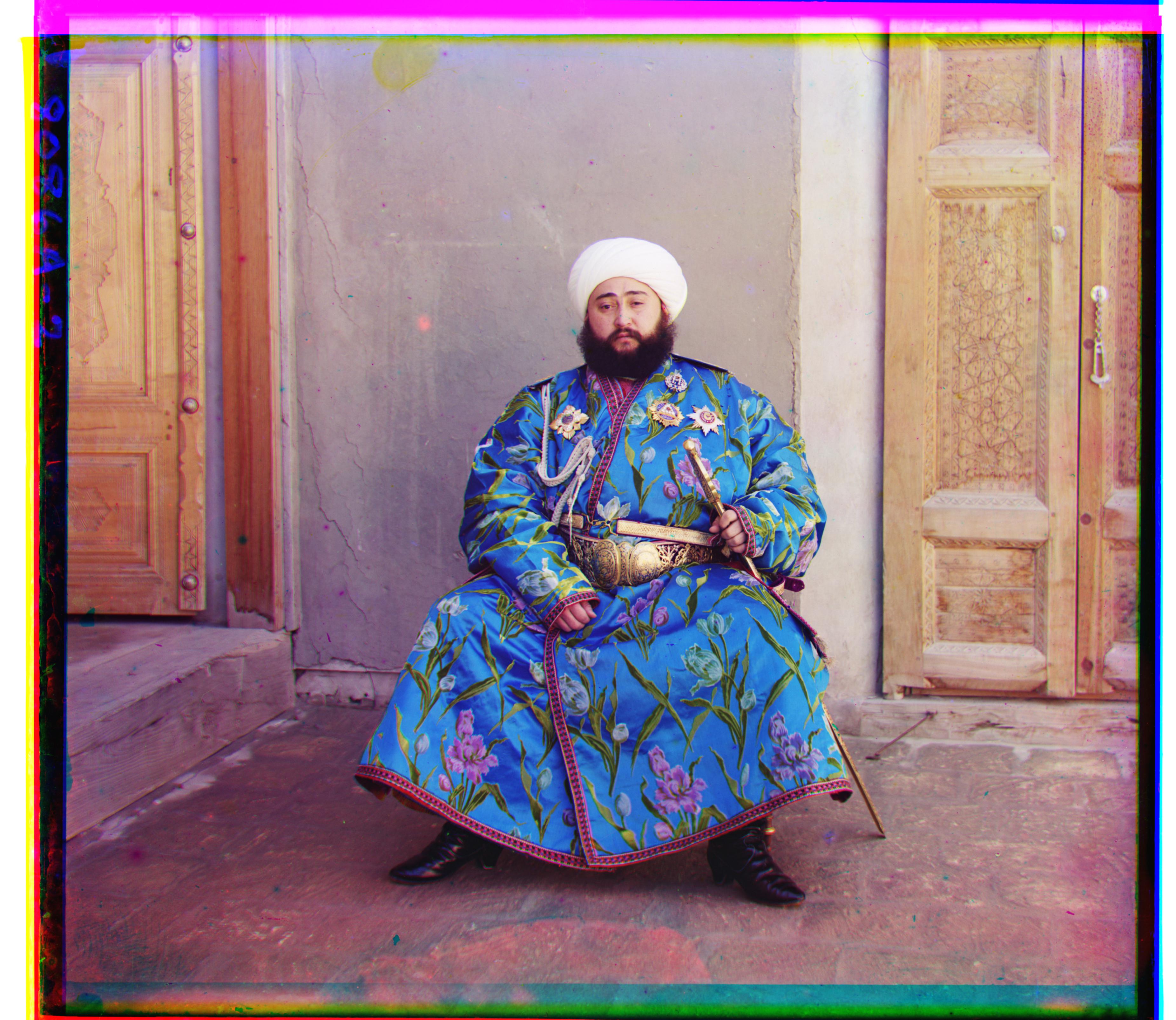
All of the bad artificats and shadow we were seeing previously have disappeared. This was a pretty great improvement.

*Object Detection

I explored one other potential method for alignment: object detection. Thinking about how edges provided good semantic information about the contents of the image to help with alignment, I wanted to see if there could be a more targetted approach using object detection. My goal was to use some out-of-box object detection model to locate the most prominent objects in each image and then simply align the bounding boxes or object centers. However, the models I looked at were all trained on just RBG images and didn’t perform too well on the grayscale color plates. Often, it was the case that only objects would be detected in a single channel, not all three. So, this proved to be a deadend, unfortunatly.

I didn’t feel the need to explore any other features for aiding in alignment since I was happy with all of the outputs at this point.

However, while the alignment was now solid, the image quality still had room for improvement. There are two main ways I went about improving the images: automatic cropping of the borders and automatic white balancing.

Automatic Cropping

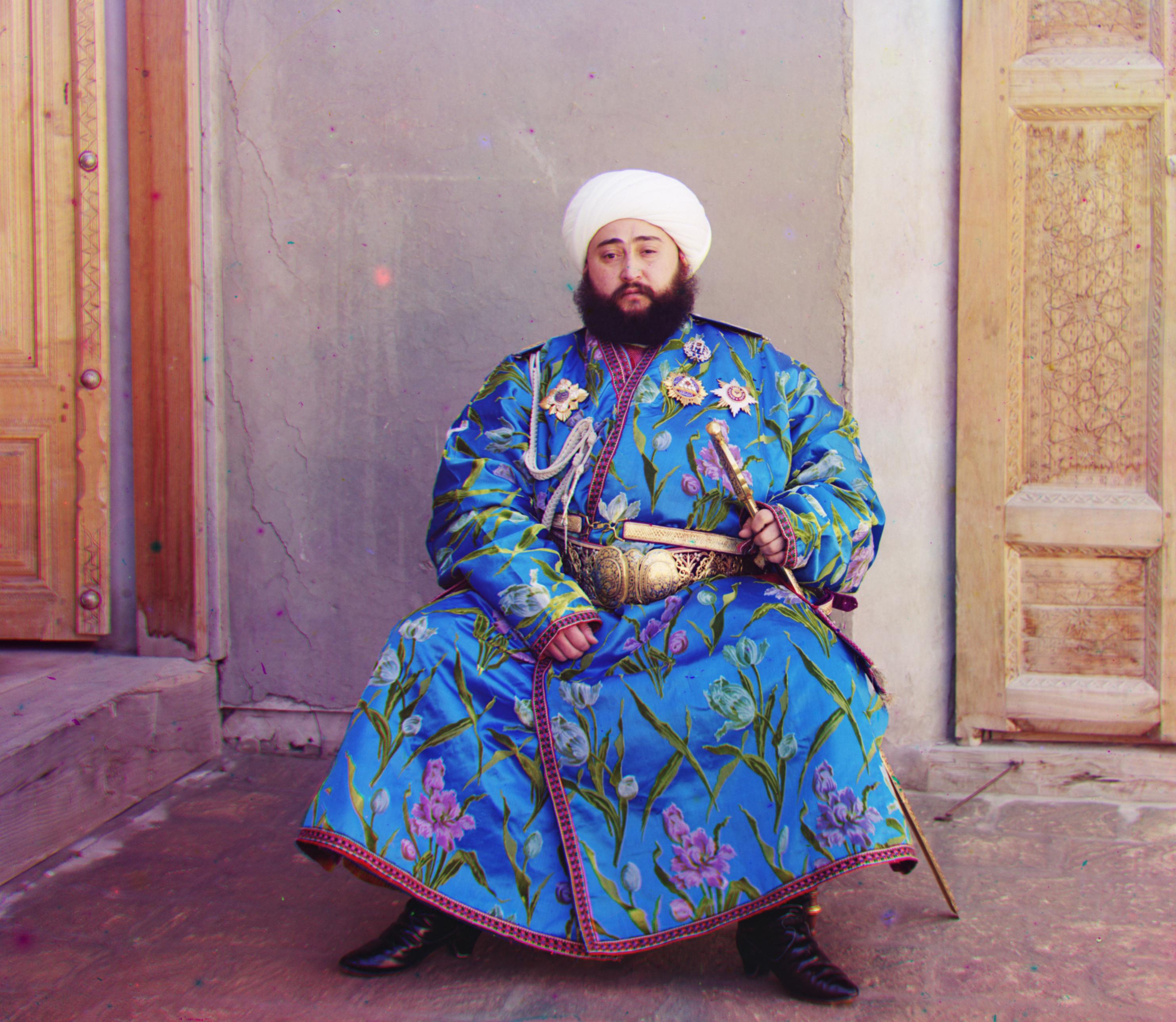
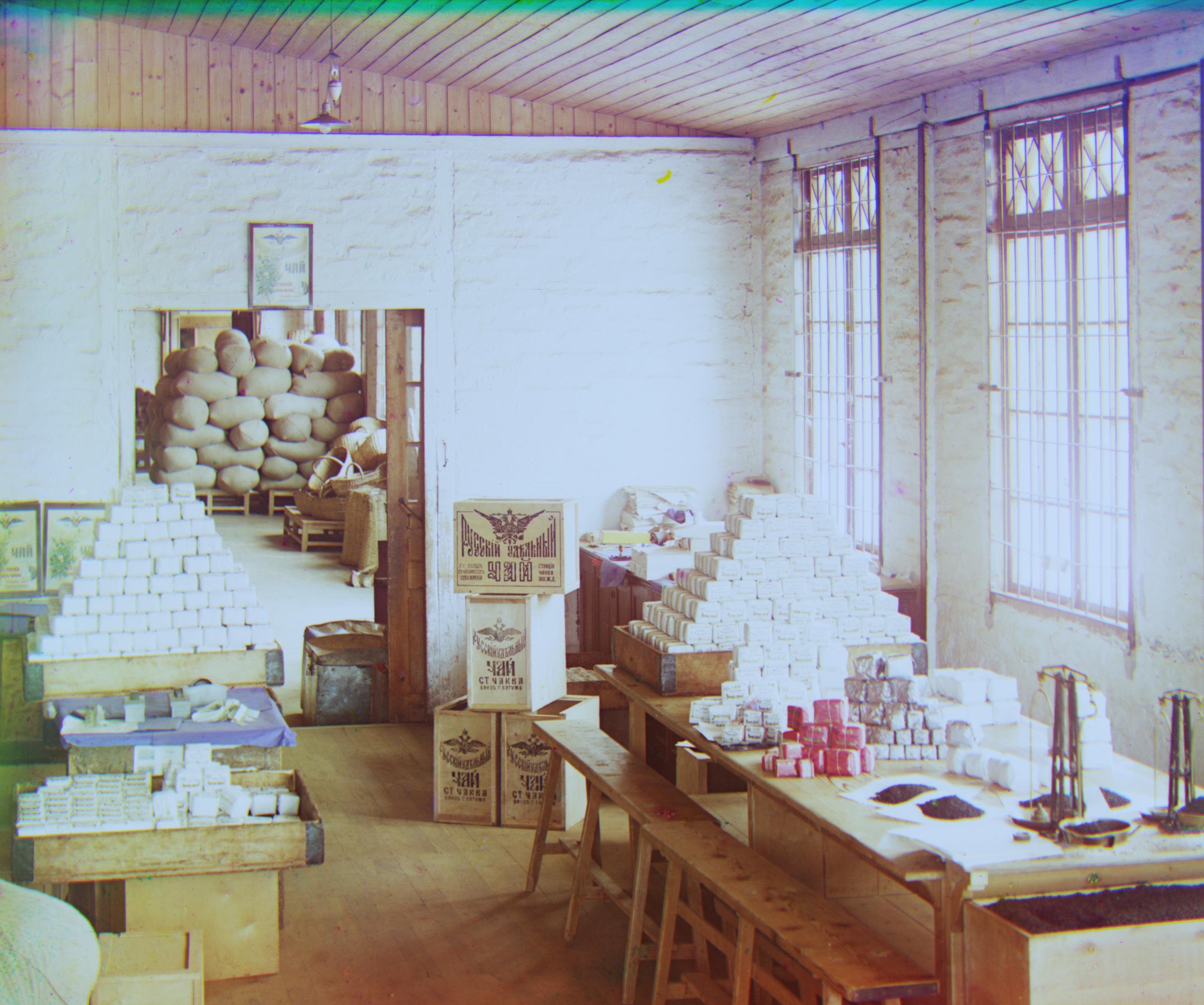
In the previous outputs, you can notice that the edges of the images aren’t very appealing and are just bars of certain colors. This is a result of the alignment process where we just rollover edges. We can also see these borders in the original color plates. Ideally, we would want to just have the main contents of the image. So, I wrote a heuristic to enable automatic cropping of the image. I used the opencv implementation of probablistic Hough Lines to find vertical and horizontal lines in the image. These lines would correspond to these borders that we are trying to get rid of. Running the Hough Lines algorithm on each color channel we can find the coordinates to crop at. However, it is possible that there are multiple lines that are detected in the image, some of which might be in the main body. To solve this, I take the maximum x coordinates in the first 10% of the image for the left side crop, the minimum x coordinates in the last 10% of the image for the right side, the maximum of the y coordinates in the first 10% of the rows in the image for the top side crop, and the minimum y coordinate in the last 10% of the rows in mage for the bottom side crop. This was a pretty effective heuristic that got mostly got rid of the color bars without cutting out much of the main image:

Automatic White Balancing

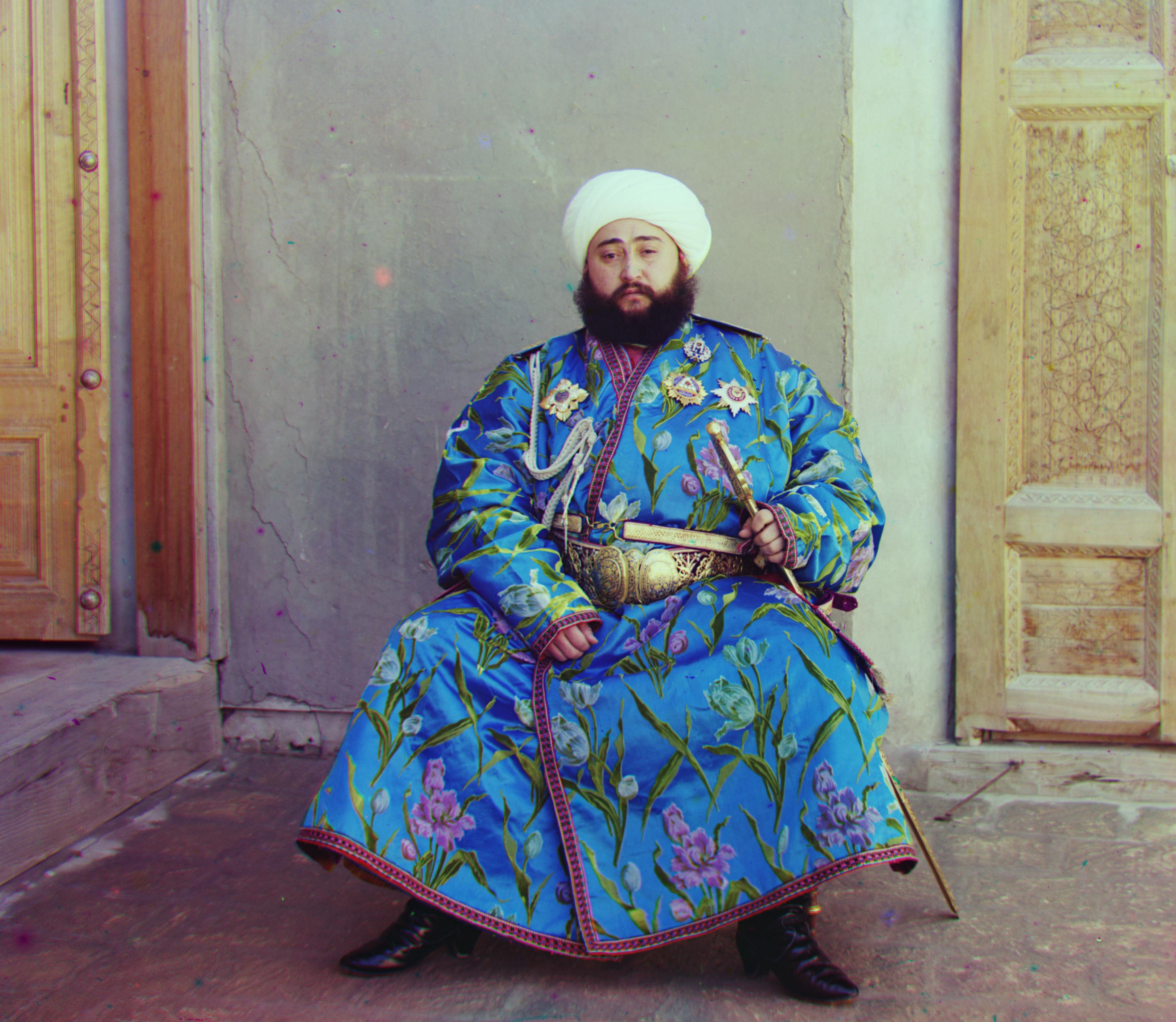
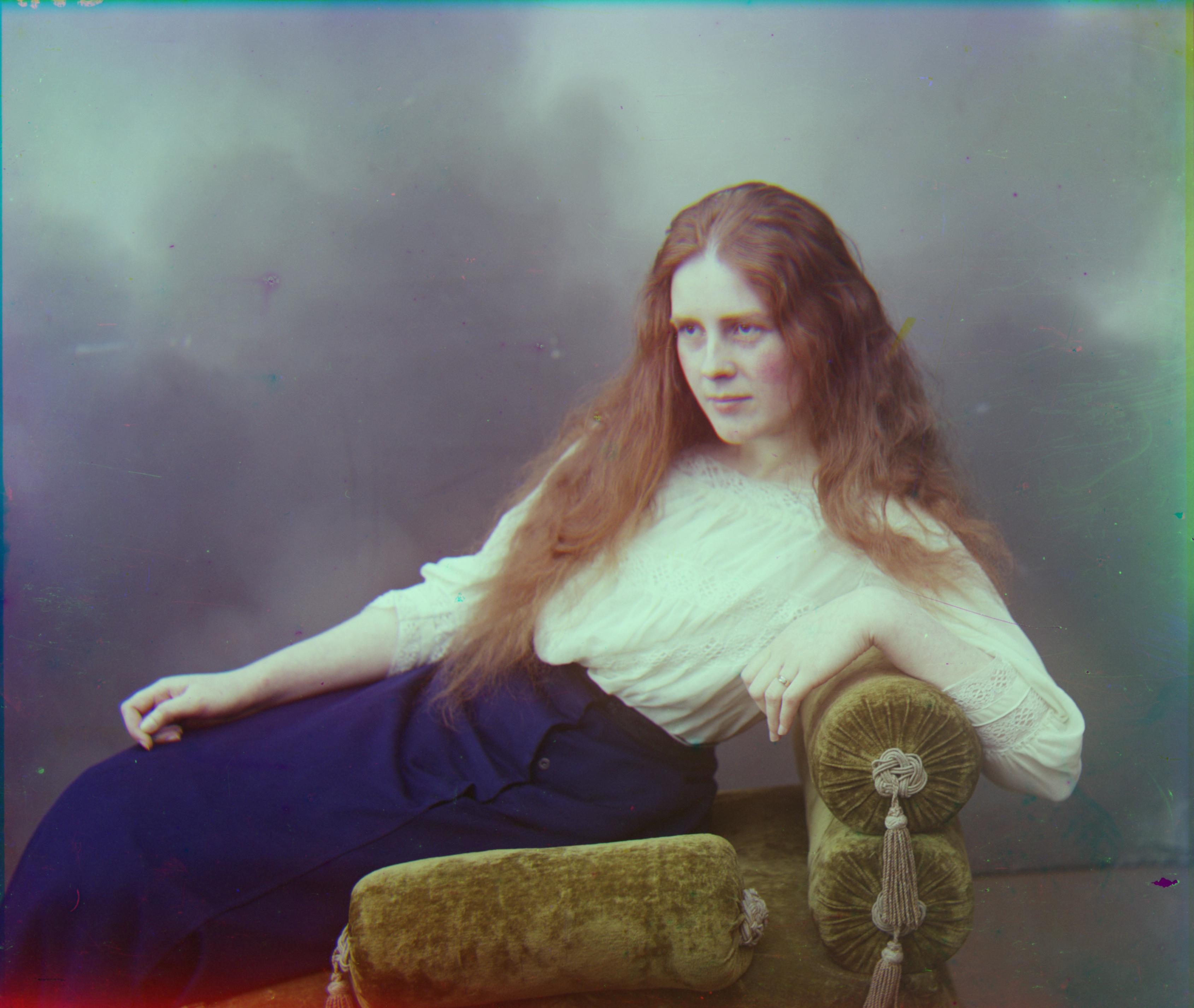
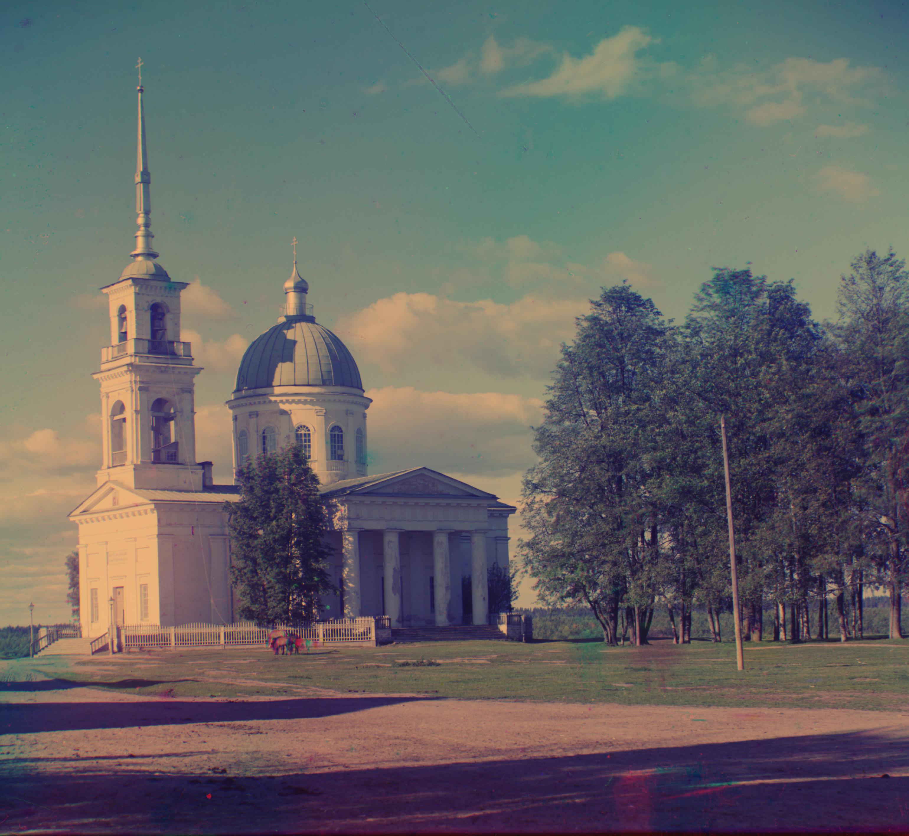
Lastly, I noticed the images were often pretty saturated with some colors appearing really strongly in the final image. So, I decided to fix this issue with white balancing. I used the opencv GrayWorld WhiteBalancer to set the average of all pixels in the image to be gray. This helped produce a more natural color tone to the image:

All Outputs

Hope you enjoyed my walkthrough for this project. I had a lot of fun trying out these various methods and seeing what worked and what didn’t. Hope you found these explanations insightful. Enjoy all of these images!

Green Channel Offset: (5, 2) Red Channel Offset: (12, 3)	Green Channel Offset: (25, 3) Red Channel Offset: (58, -4)
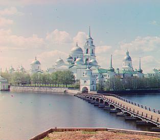
Green Channel Offset: (49, 24) Red Channel Offset: (107, 40)	Green Channel Offset: (60, 18) Red Channel Offset: (123, 13)
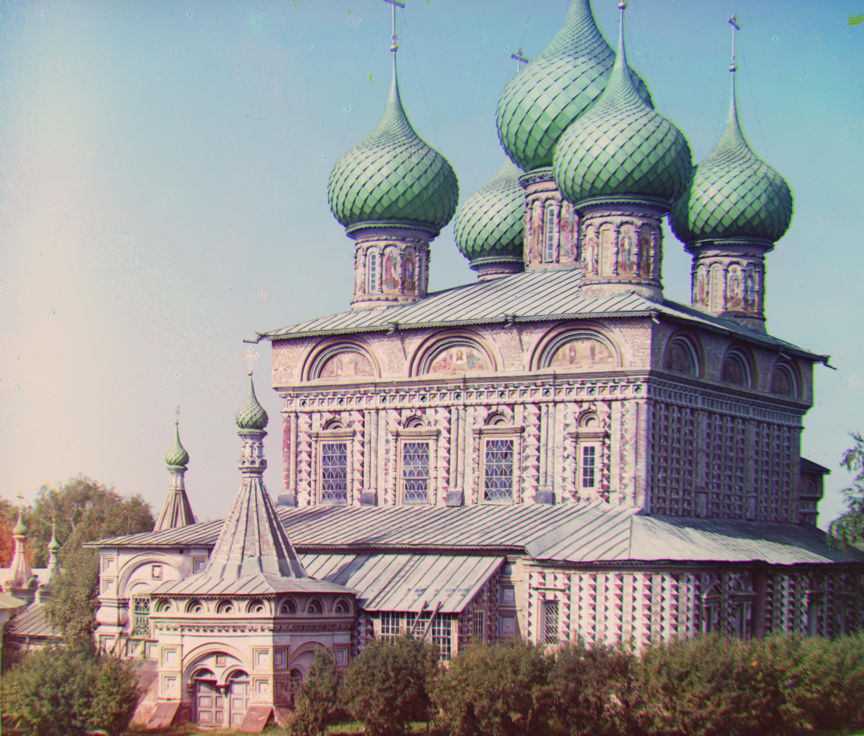
Green Channel Offset: (40, 16) Red Channel Offset: (89, 23)	Green Channel Offset: (56, 10) Red Channel Offset: (120, 13)
Green Channel Offset: (80, 10) Red Channel Offset: (167, -6)	Green Channel Offset: (-3, 2) Red Channel Offset: (3, 2)
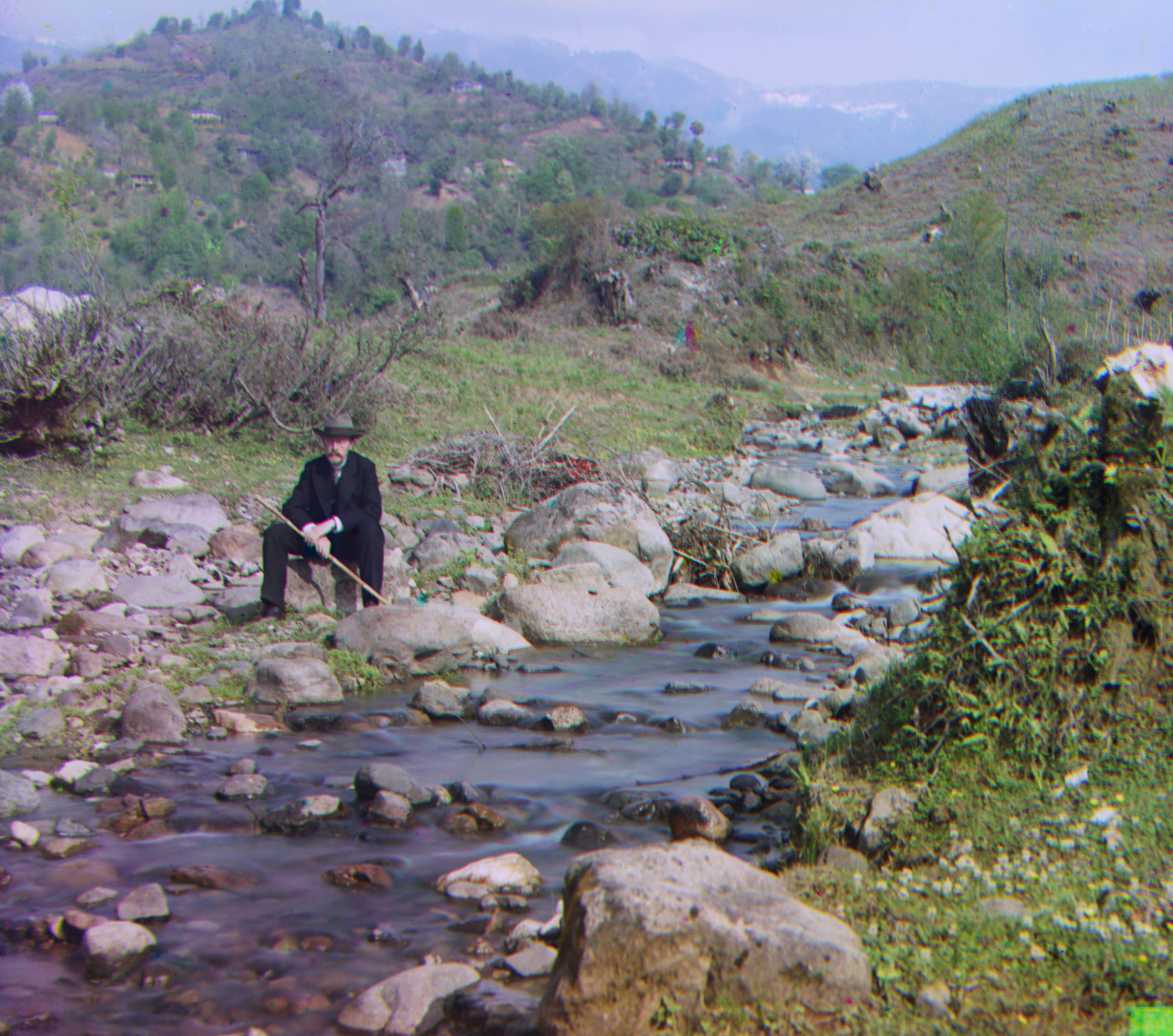
Green Channel Offset: (52, 24) Red Channel Offset: (110, 36)	Green Channel Offset: (77, 29) Red Channel Offset: (170, 35)
Green Channel Offset: (54, 17) Red Channel Offset: (113, 11)	Green Channel Offset: (3, 3) Red Channel Offset: (7, 3)
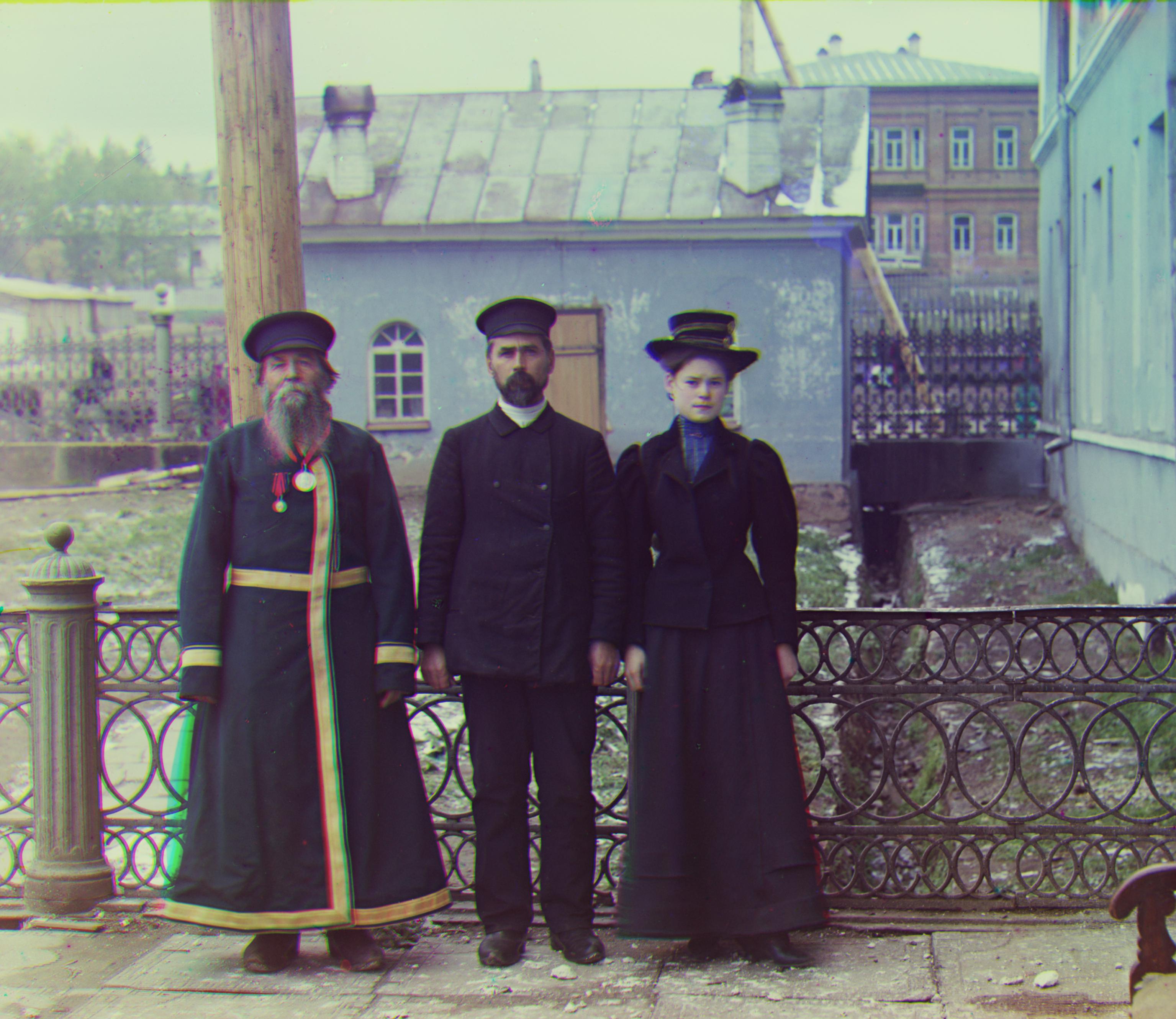
Green Channel Offset: (43, 7) Red Channel Offset: (85, 29)	Green Channel Offset: (53, -1) Red Channel Offset: (105, -12)
Green Channel Offset: (25, -12) Red Channel Offset: (98, -21)	Green Channel Offset: (58, -12) Red Channel Offset: (135, -55)