
|

|

|
Segei Mikhailovich Prokudin-Gorskii was a chemist and the first color photographer.
After receiving help from the Tzar of the Russian empire, he build a camera that took three exposures of the same scene through a red, green, and blue filters.
This captured three black-and-white photographs of the blue, green, and red frequencies of the scenery.
Although he first planned for the three images to be projected using a special projector, it never happened; however, we can now reconstruct the original scenes programmatically.
Resotring the colored photo is surprisingly simple. Since RGB is a commonly used color representation, we can treat each of the three frames as the intensities of red/green/blue, and overlay them together to restore a colored image.
Although it seems sound, the result is really blurry since the three channels are not aligned.
To fix this, we introduce ways to align the images.
We can phrase the problem of aligning the images as an optimization problem.
First you can define a goodness-of-fit metric, then the solution is the x,y offsets for each of the channels that maximizes the goodness-of-fit.
In the project, I tried L2 distance between images and normalized cross-correlation (NCC), measured as the dot product between the normalized images =im1*im2/(||image1||||image2||), and found that empirically the NCC objective produces higher quality alignments.
To solve this problem, we can naively search every possible offset within the image. This is feasible for small images, computing the NCC on which does not take long and which will naturally not have many possible offsets.
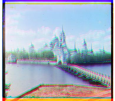
The results of regular search are displayed for small images, for which I tried offsets between -15 and 15 in both vertical and horizontal directions.
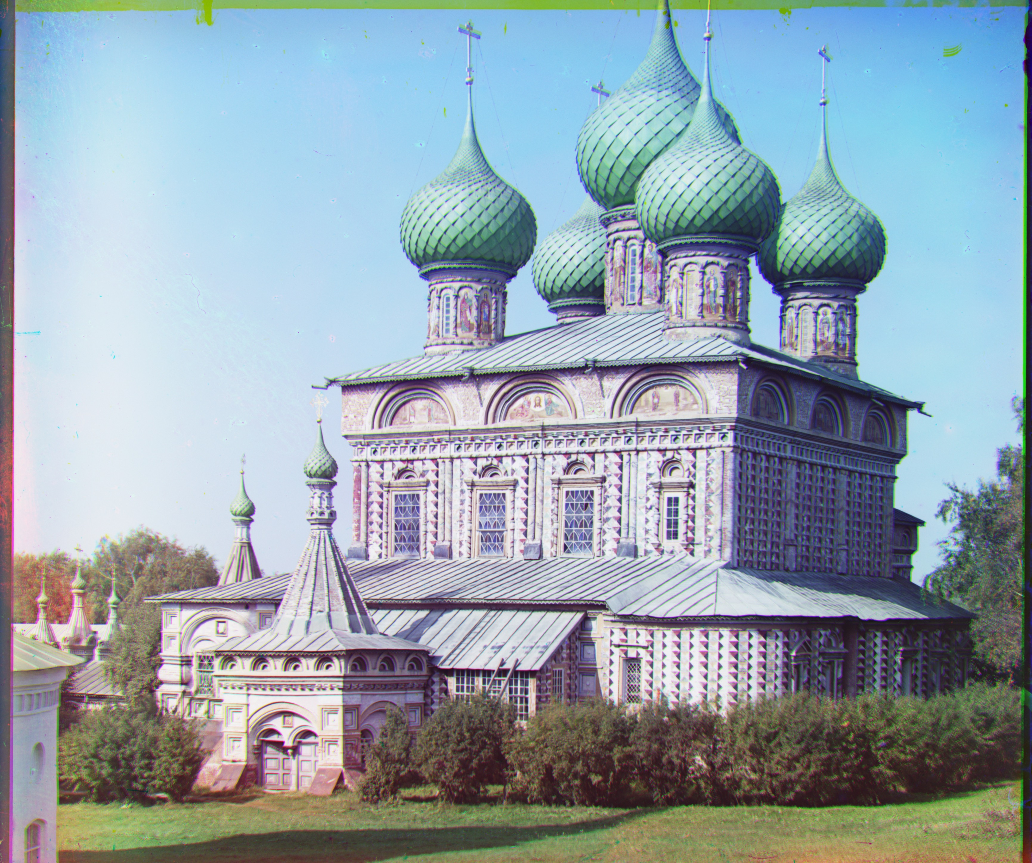
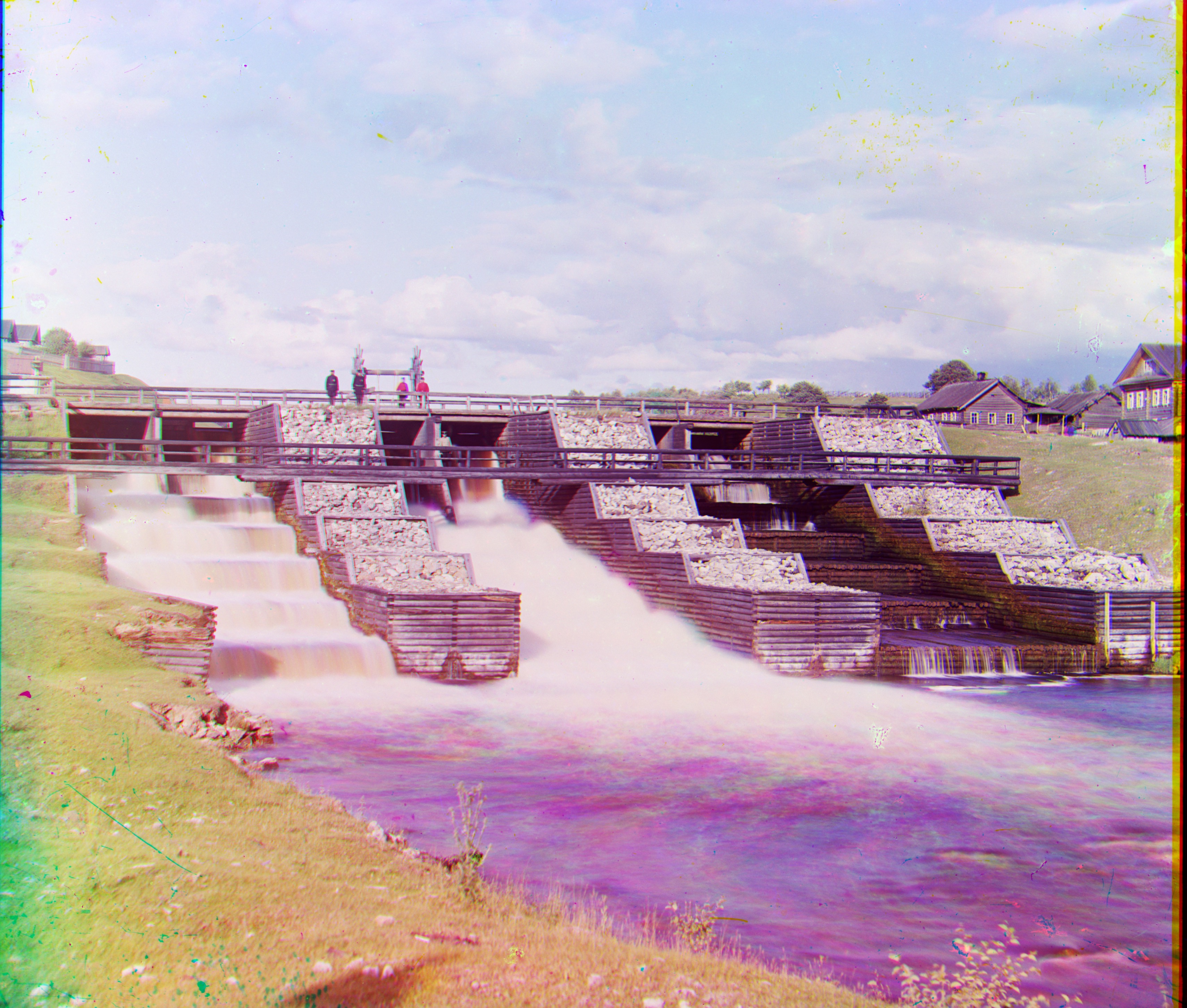
Naive search above fails on large images (over 2000x2000) because the borders can be large and the NCC operation itself becomes costly.
Rather than linearly searching all possible values of the offsets, we can treat this as a dynamic programming problem.
The key insight is that we do not need to look at the full image to decide between an offset of -64 and 64. We can downsize (an efficient operation) the image and compute the NCC on the downscaled verison.
After we have the course estimate of -64, 0, or 64 offset, we can refine it by adding -32, 0, or 32, this time looking at a slightly larger version of the image.
By repeating the above steps recursively until -1, 0, 1 offsets, we can achieve the flexibility of offsets, without computing NCC on the full-sized channels every time.
Specifically for my implementation, I downscaled the image by 0.5 if it was larger than 200 pixels and solved the alignment problem on the smaller image.
Then, I multiplied the offsets I receive by 2 to scale the offsets back up. I searched offsets of -4 to 4, which allowed the program to correct some mistakes it might have made in smaller scales by sacrificing some compute.
The above description isn't enough to implement the full algorithm. There are a few points I'd like to notes.
First of all, I aligned the red and blue channels independently against the green channel. I chose the green channel as the base empirically; however, I supposed that it covers a lot of high-texture wildlife elements, making it a good basis.
Although aligning them independently may cause the red and blue channel not be optimally aligned, this was a good trade-off in complexity.
Secondly, I cropped 5% of the image on each side throughout each alignment computation. This easily discarded most of the borders and drastically improved the alignment results.
Lastly, I implemented automatic contrasting for all of the images below in two different ways.
First was treating each channel individually, and computing new channel intensity as =(value-min)/(max-min).
The other way was treating channels together and computing new pixel as a vector =(pixel-min_pixel_norm)*(sqrt(3)/(max_pixel_norm - min_pixel_norm)). All of the below images have been contrasted using the latter technique.
|
|
|
|

|

|

|
|
|

|

|
|

|

|

|

|

|

|
|