|
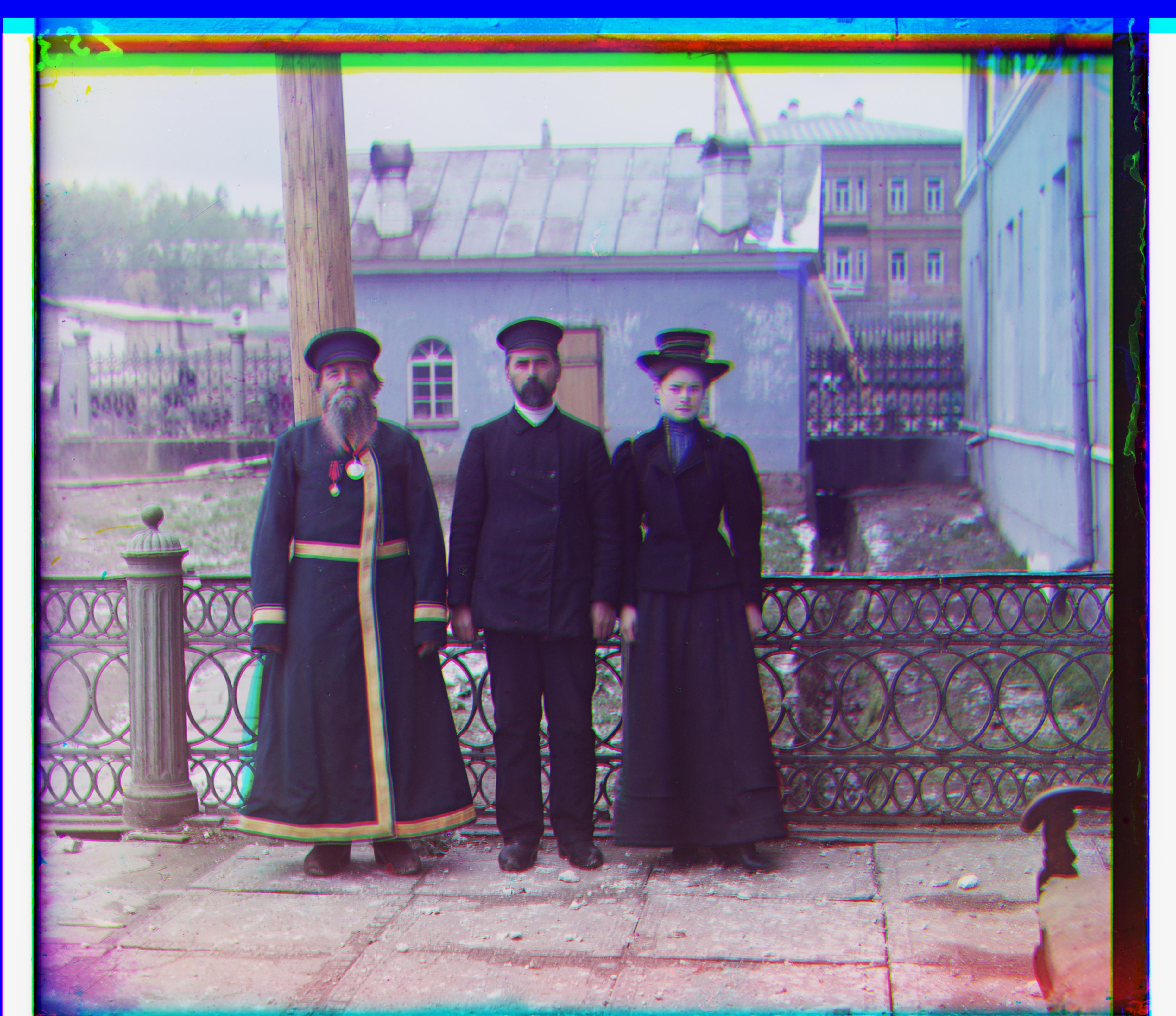
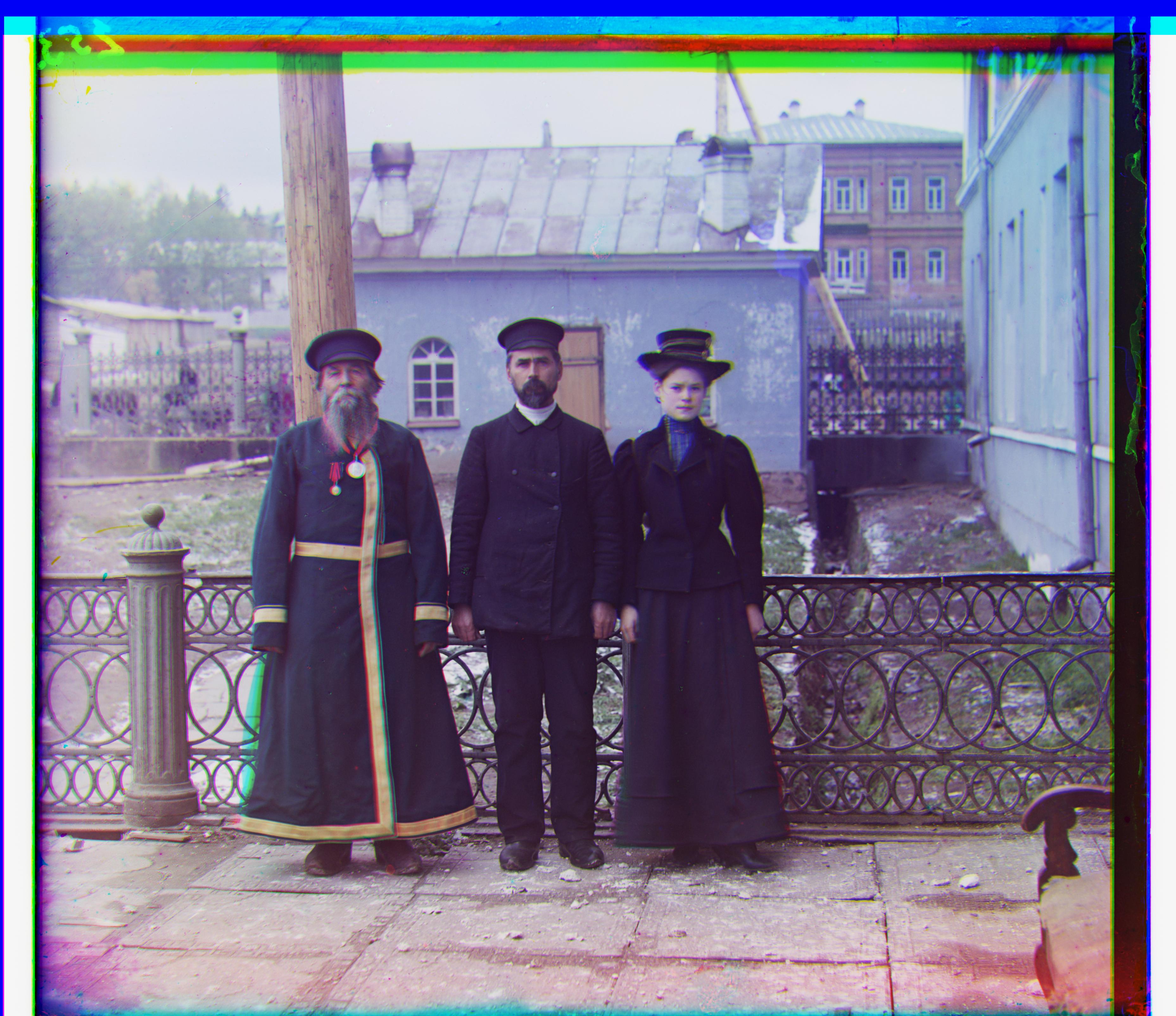
Standard method using all pixels |
Using only edge features |
|

|
|
|
|
|
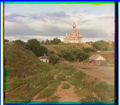
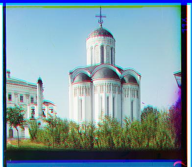
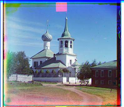
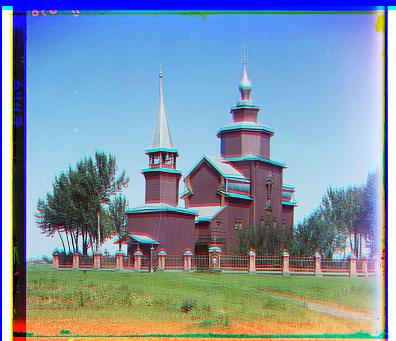
This project's goal is to combine the glass plate negatives from the Prokudin-Gorskii collection to reconstruct a RGB color image.
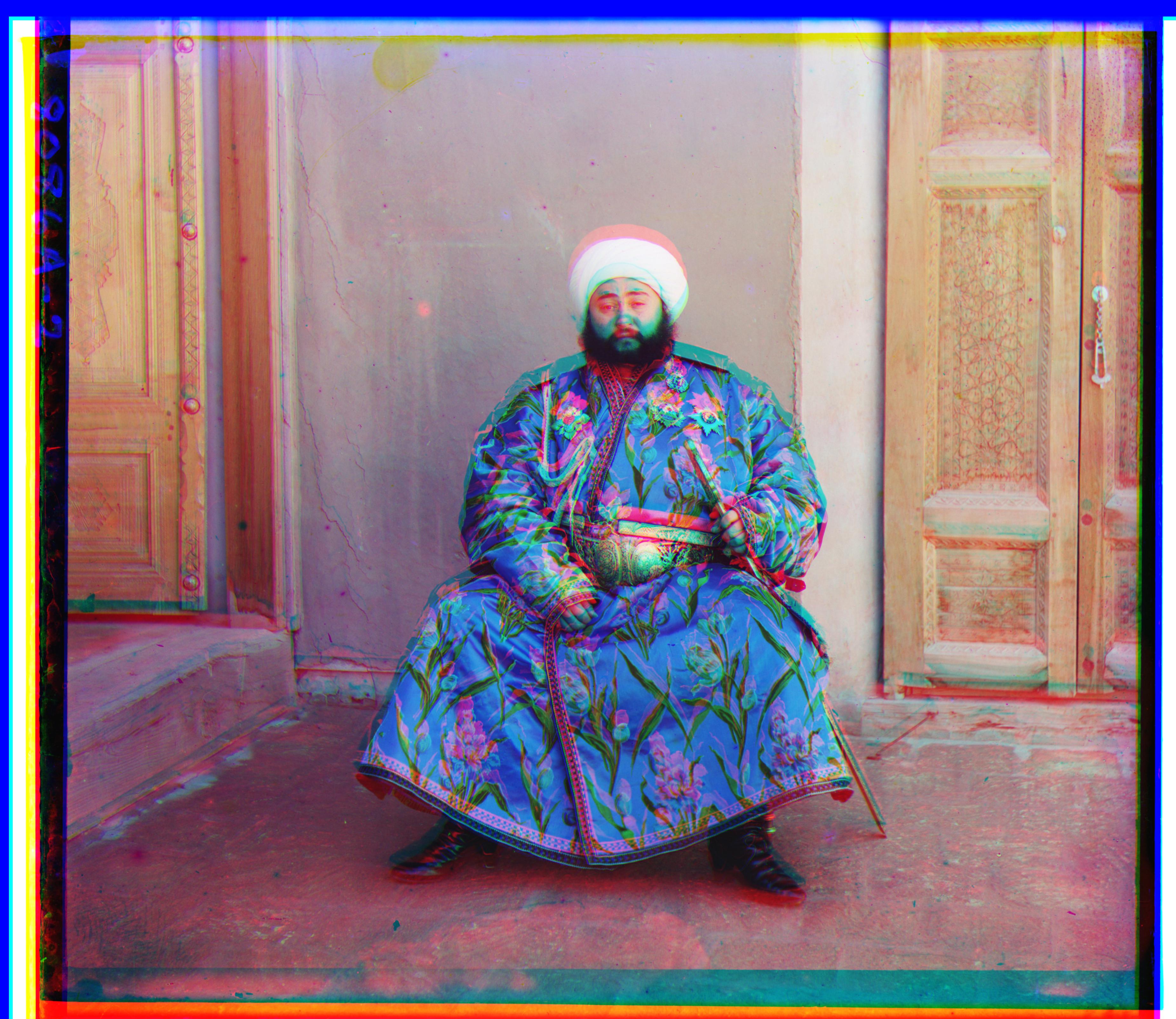
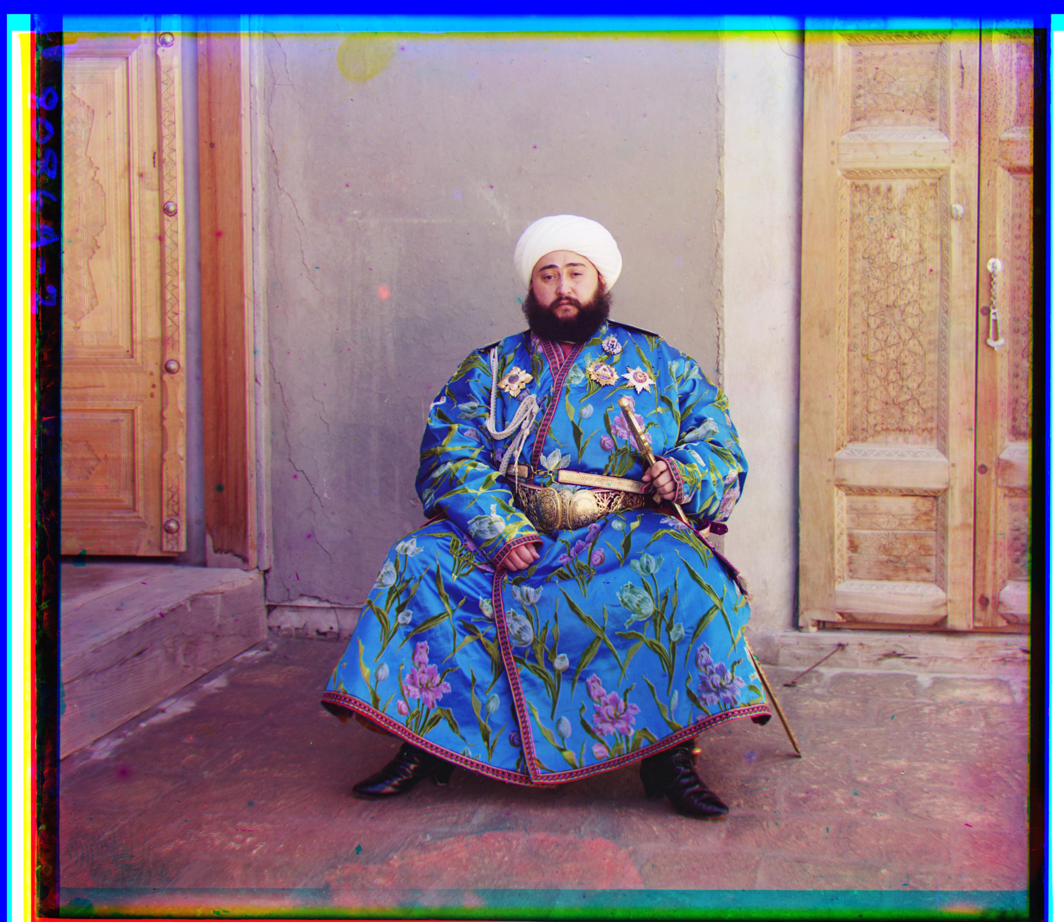
To align the red and green channels to the blue channel, I perform an exhaustive search by trying to shift the red/green image to match the blue image. First, I shift the red/green image for every value in the range [-12, 12] in both the x and y directions. After I shift the image, I crop the outer 20% on all edges of the image to remove the border, as the border when included in the similarity metric makes the metric less accurate. Finally, I use the Sum of Squared Differences for the similarity metric, which tries to minimize the Frobenius norm of the shifted image minus the blue image. For bells and whistles, I found that just relying on the RGB pixel intensities to match when calculating similarity was not at all accurate. Instead, I extracted edge features from the images by combining a Gaussian blur and the Canny edge detector. Then, the standard exhaustive search is just run on these edge images, which only keeps the important information of the image. Examples of both methods are shown below.
|
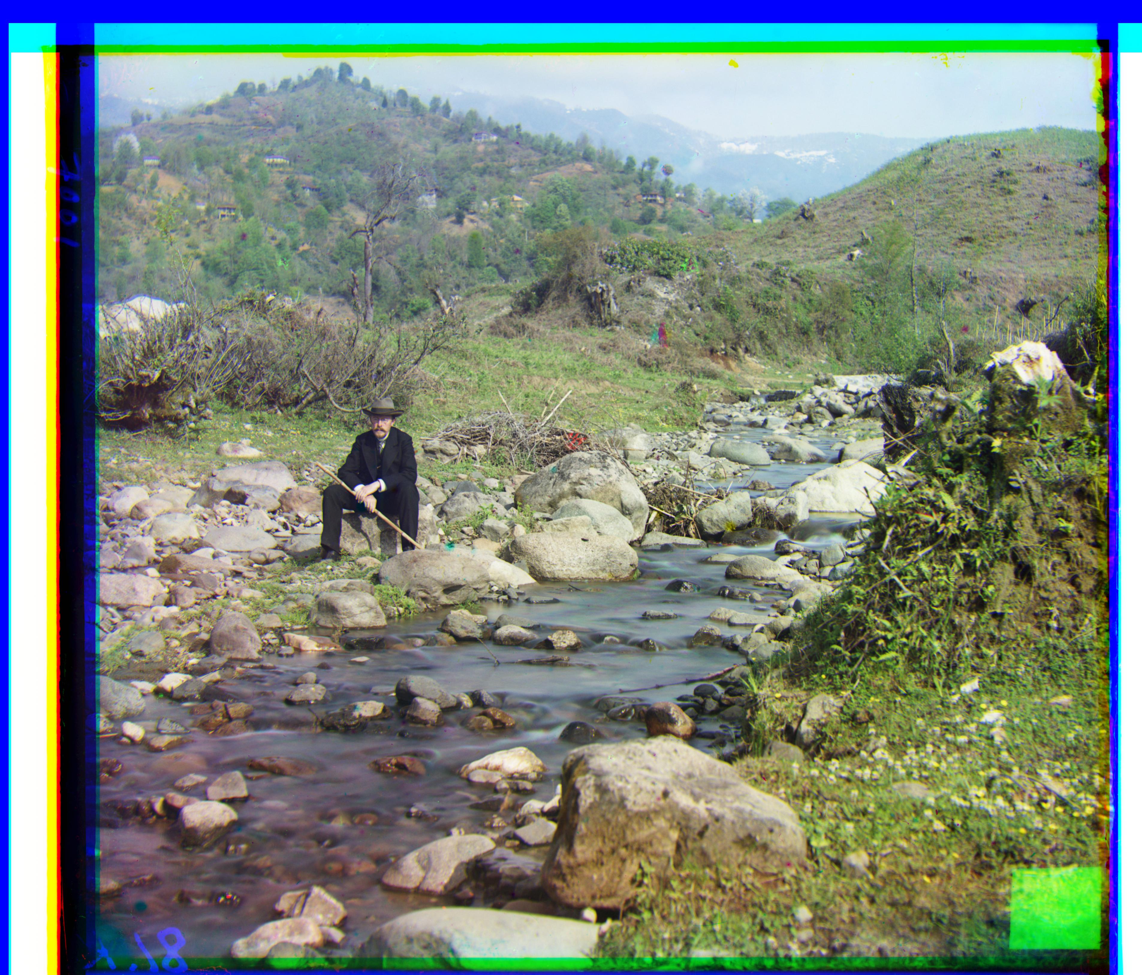
Standard method using all pixels |
Using only edge features |
|
|
|
|
|
|
|
|
|
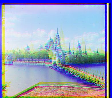
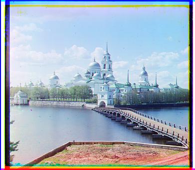
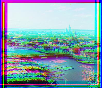
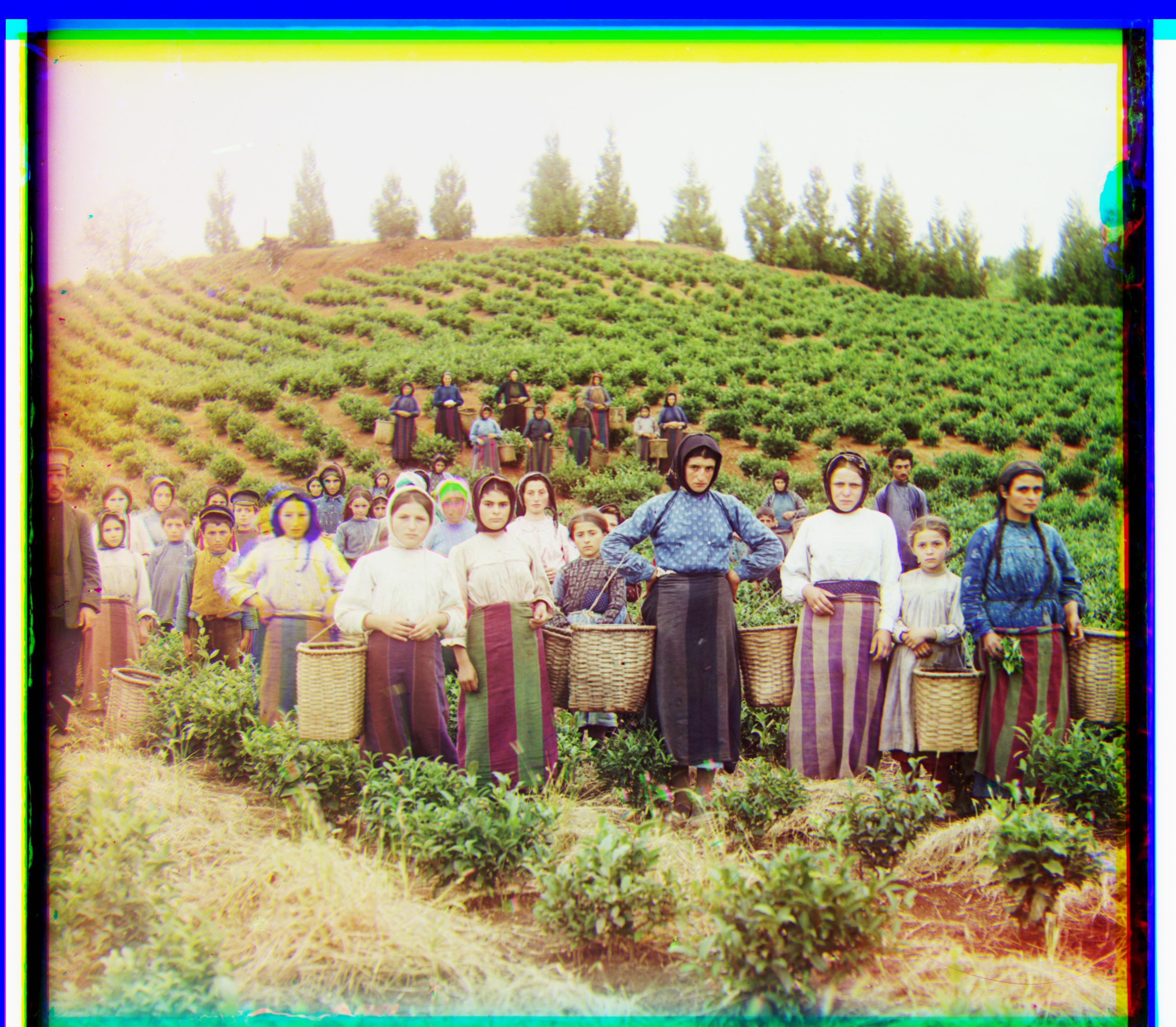
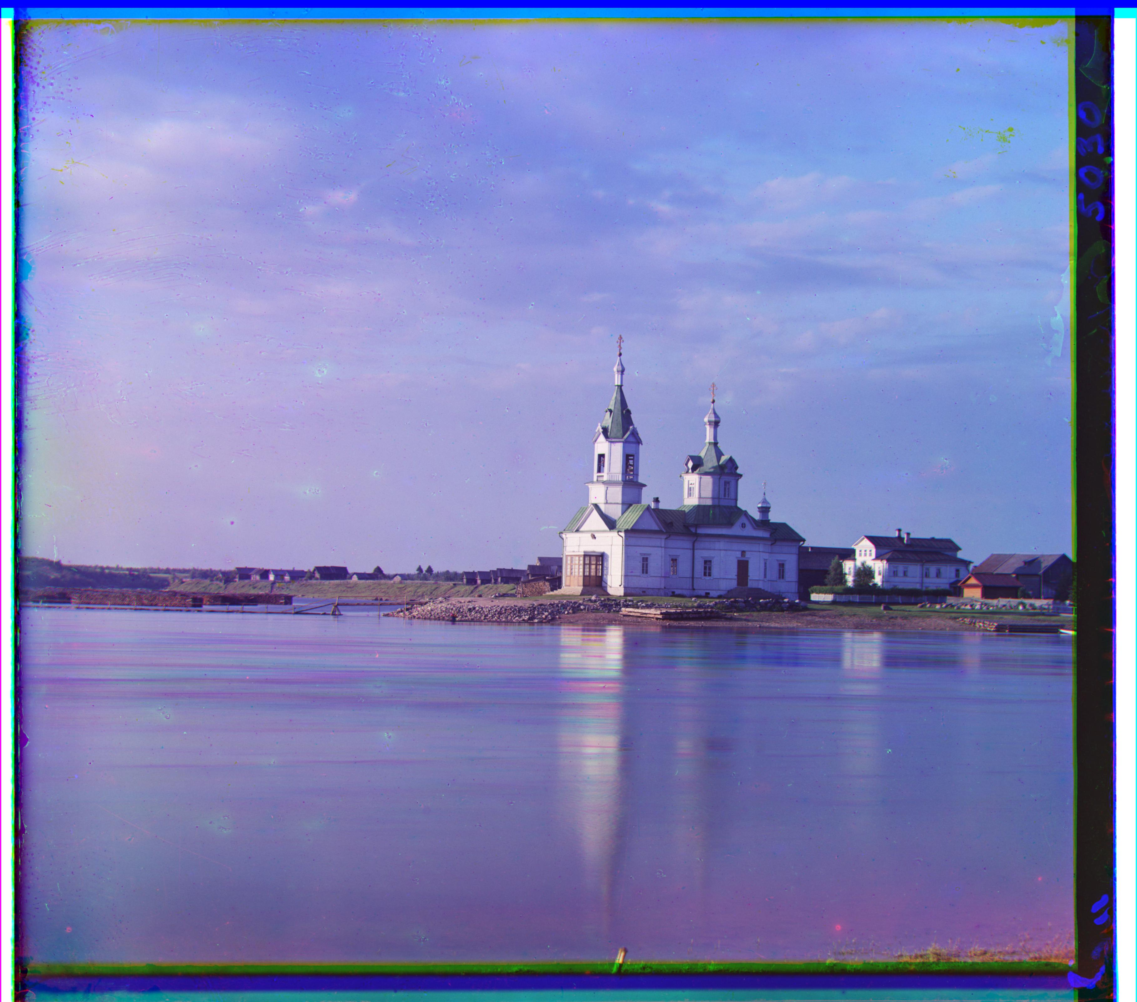
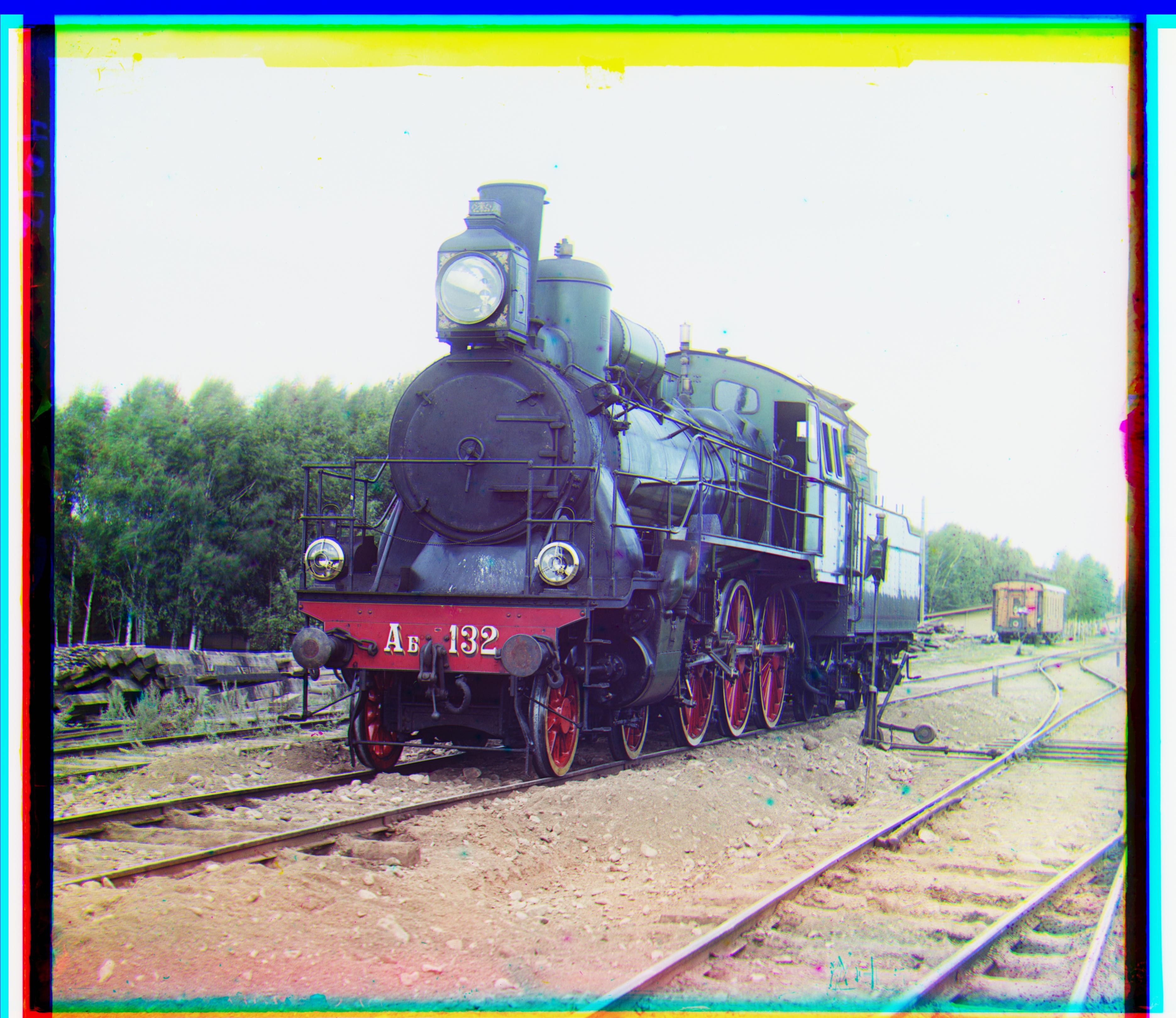
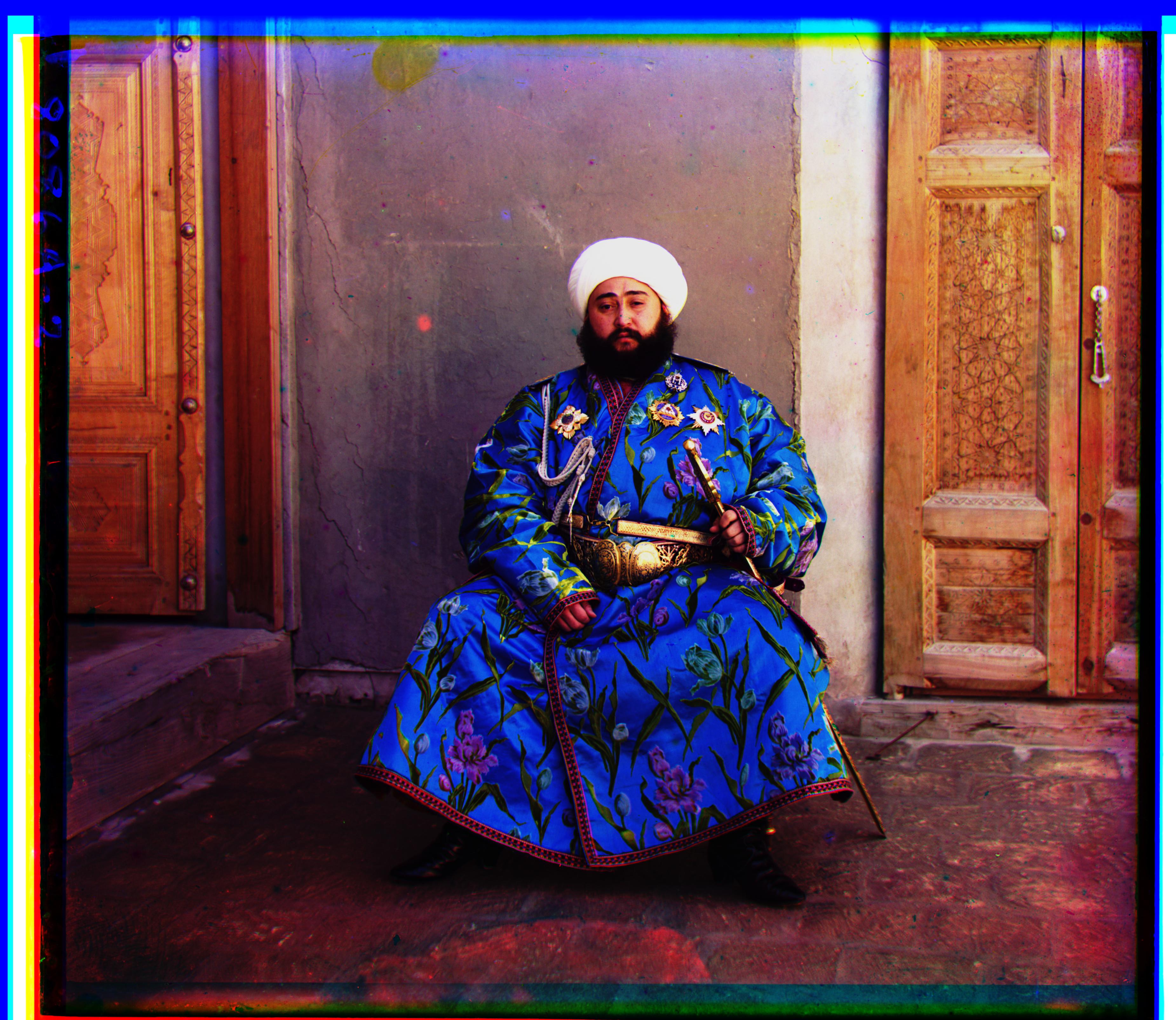
While the exhaustive search will work for small JPG images, it will be extremeley slow for large TIF files. To speed up our computation, I implemented an image pyramid that looks at images at various resolutions. Each level up the pyramid was 1/2 as large as before, and was downsampled while accounting for anti-aliasing using the sk.transform.rescale function. We keep on downsampling till we get to an image that has less than 100 pixels, after which the standard exhaustive search from the previous part is used. Then, as we go back down the pyramid, before doing the exhaustive search, we need to multiply the previous offset by 2 to account for the downsampling. Since we are using an image pyramid and the offsets at the small resolutions get amplified later, we only need to check shifting in the range [-5, 5] in the x and y direction at all levels of the pyramid. The bells and whistles method of using the edge features to calculate similarity doesn't improve the performance as much as before, probably due to the image pyramid which allows for more fine tune shifting of the image channels. The only exception is the emir photo which is significantly better when using edge features.
|
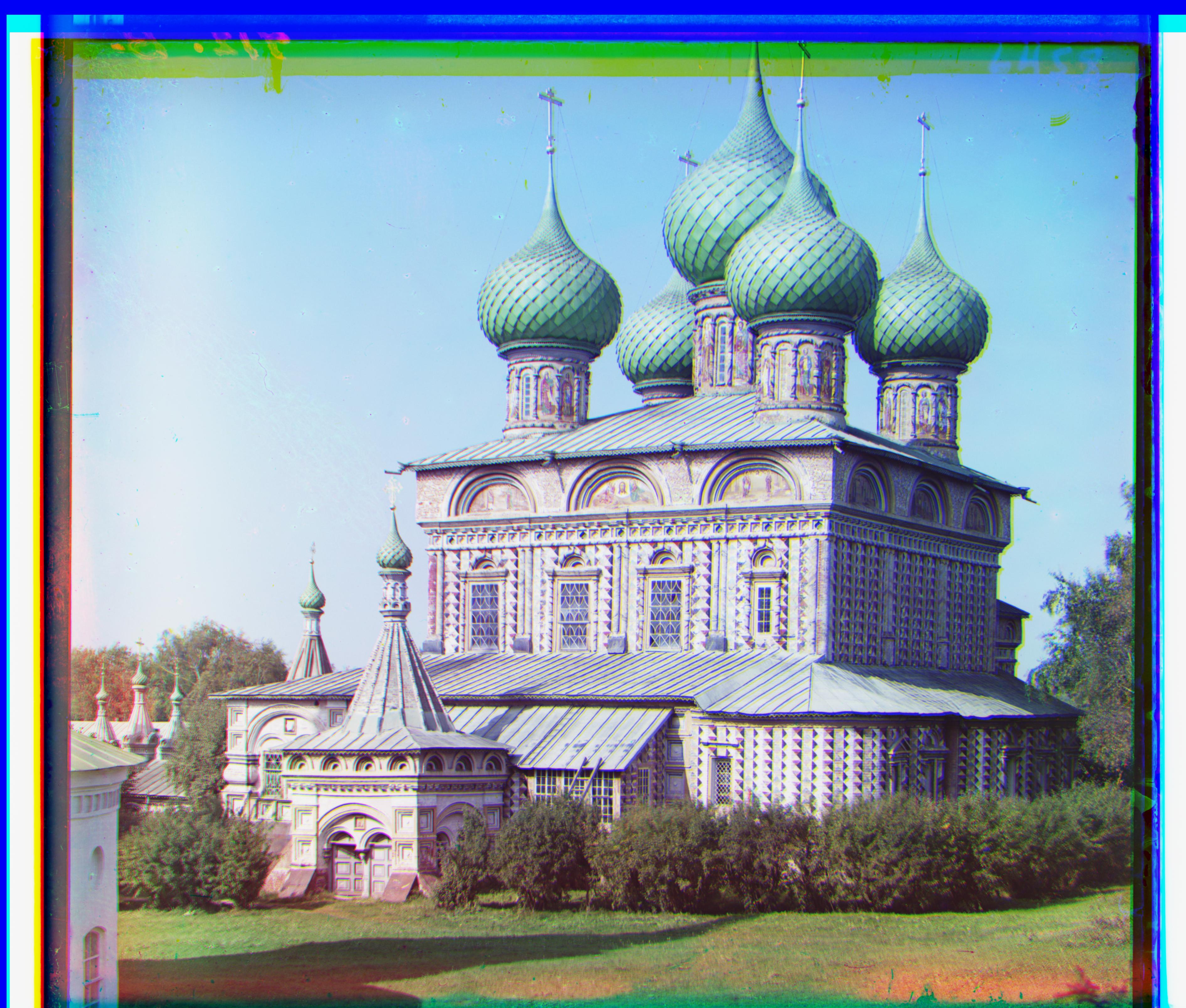
Standard method using all pixels |
Using only edge features |
|
|
|

|
|

|
|
|
|
|

|
|
|
|
|
|
|
|
|
|
|
|
As mentioned earlier, since using all the pixels for similarity measurement produces incorrect shifts, especially when channels have different intensities, I instead only used the edge features of the shifted color channel when calculating the similarity metric. This was done by combining a Gaussian blur (convolution with Gaussian kernel) to remove high-frequency features and then the Canny edge detector to extract the edges from the image. The images showing the comparison are already above.
Additionally, I implemented automatic contrasting using the histogram equalization algorithm lecture. It works by first converting the RGB image to an HSV image, so we can just use the value of the pixels as the intensity. Then, we create a cumulative histogram of the all the pixel values and scale it from 0 to 1 to act as a CDF. Then we can use a fact from probability theory that applying the CDF will produce a uniform distribution over the pixel values. Some examples of the automatic contrasting are below, and it can be seen that the contrast is often extreme.
Automatic Contrasting with Histogram Equalization
|
|
|
|
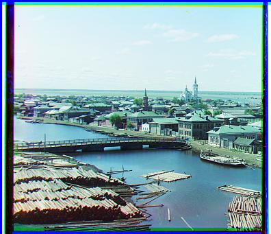
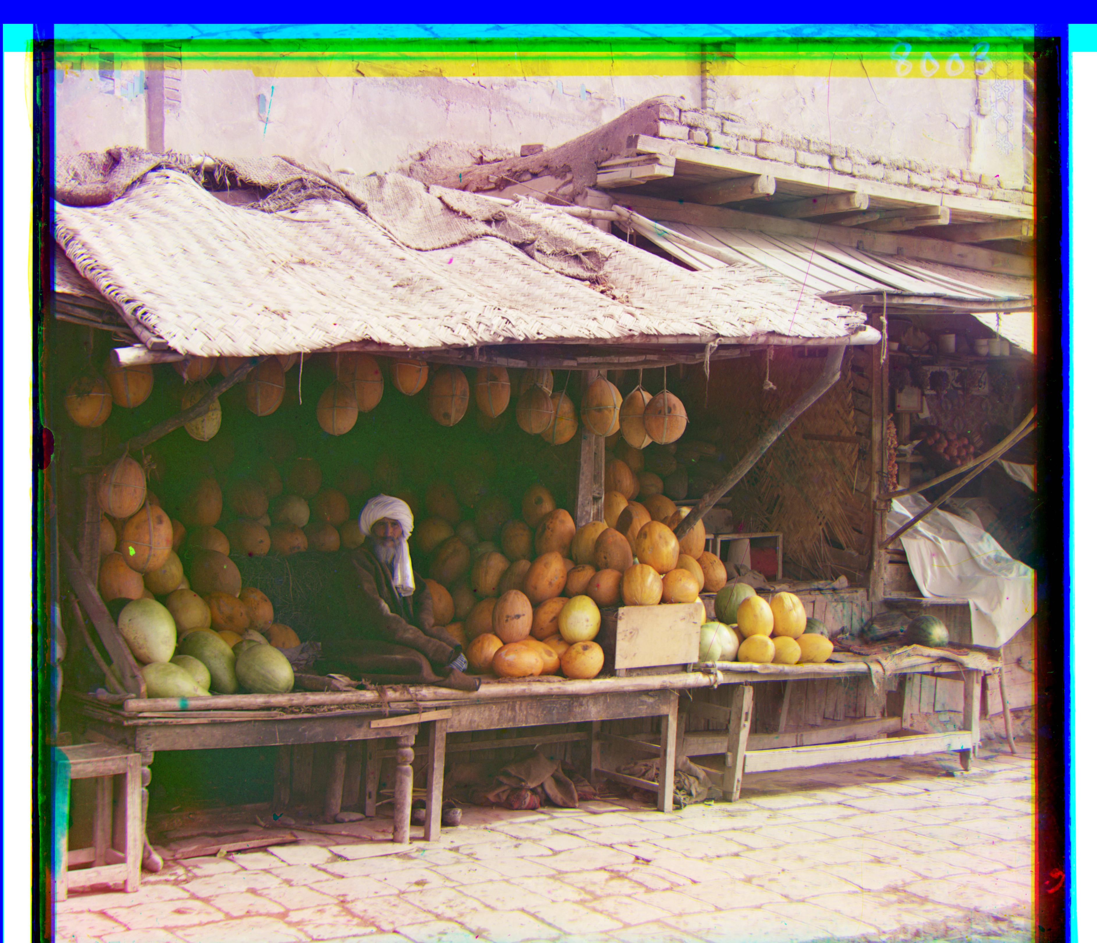
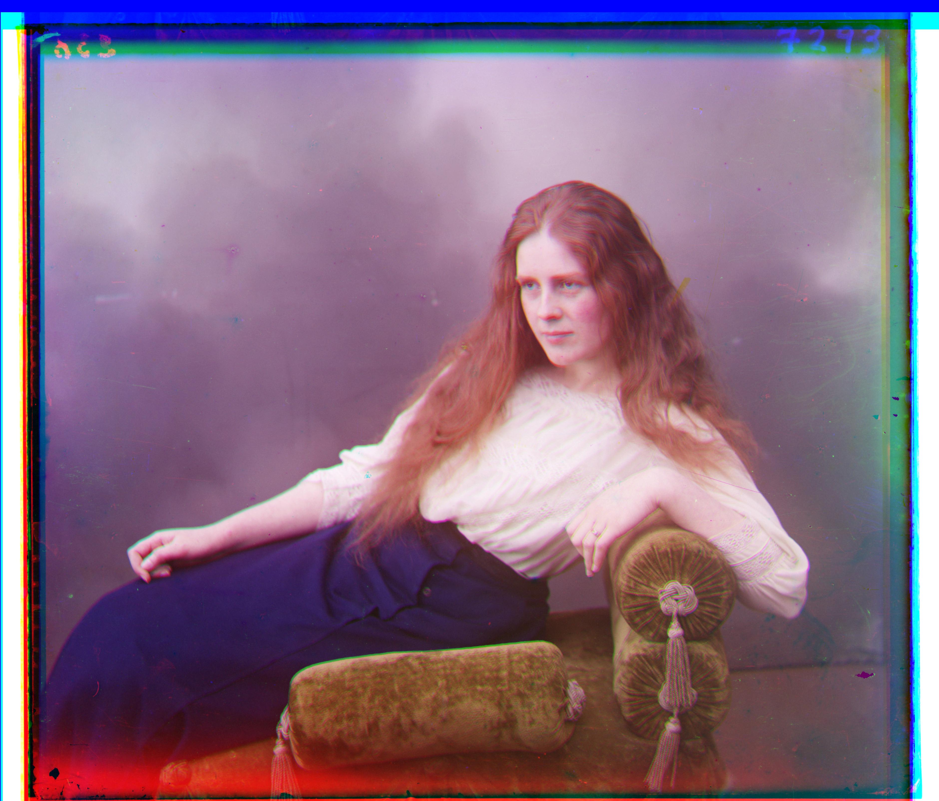
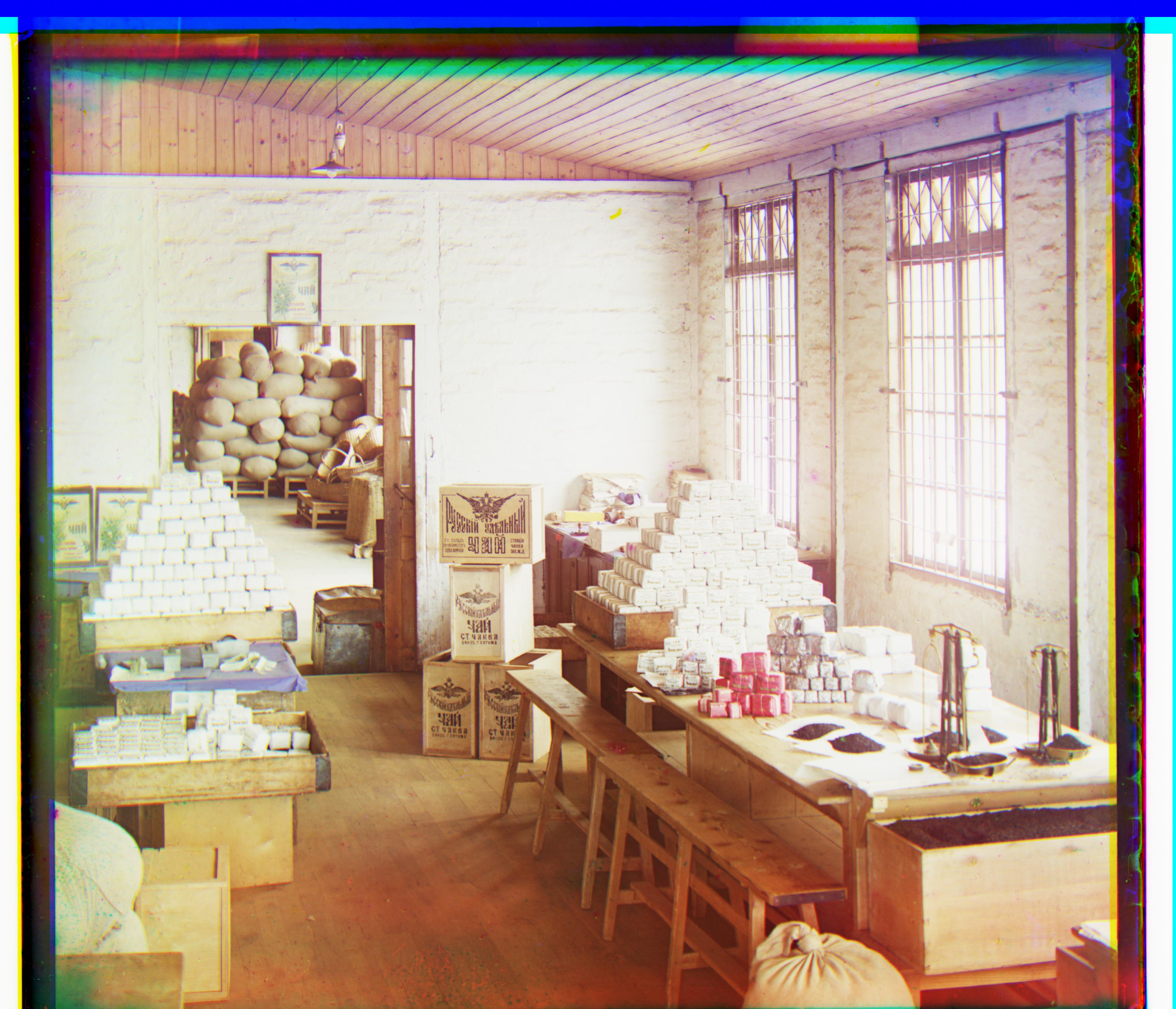
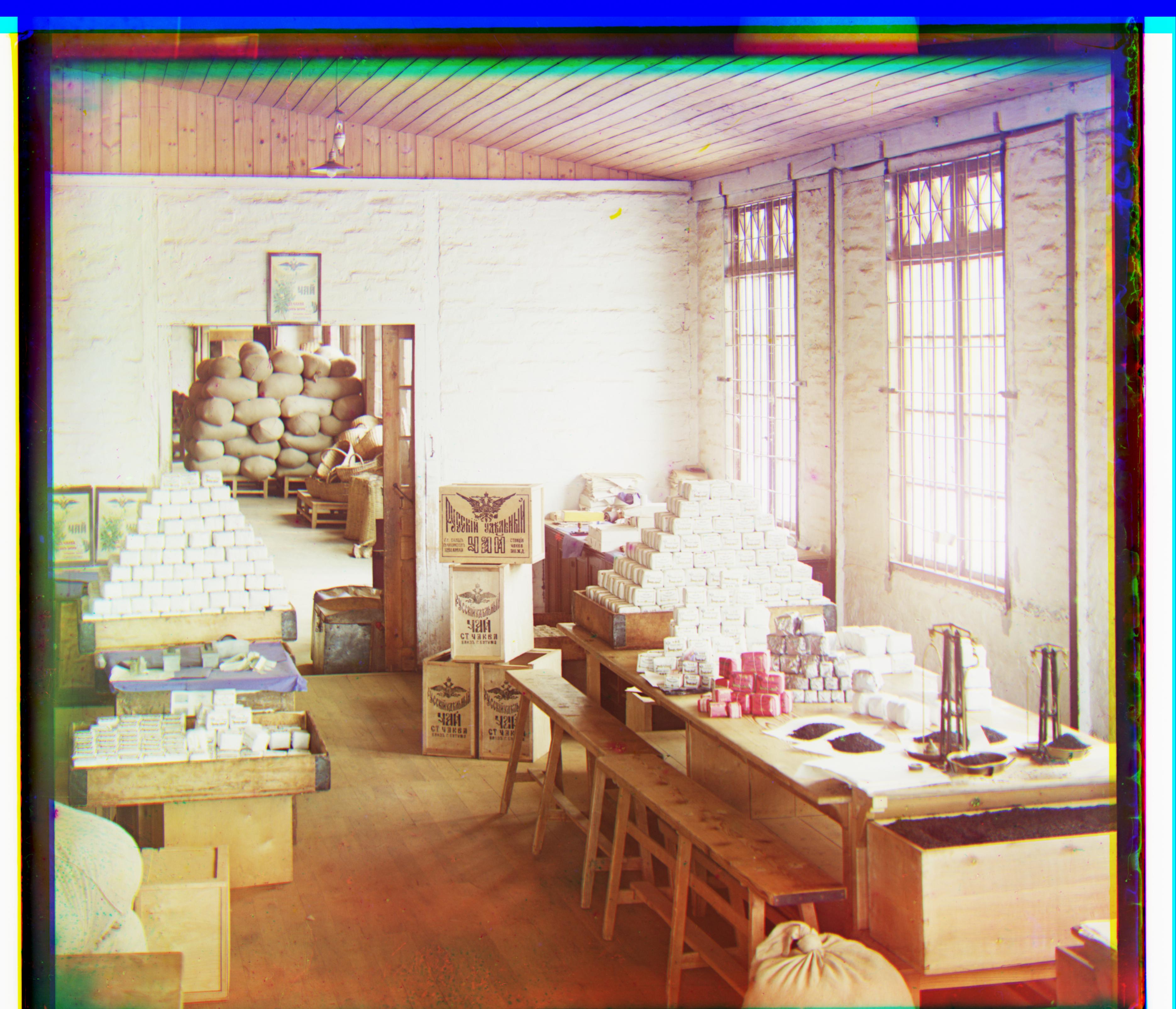
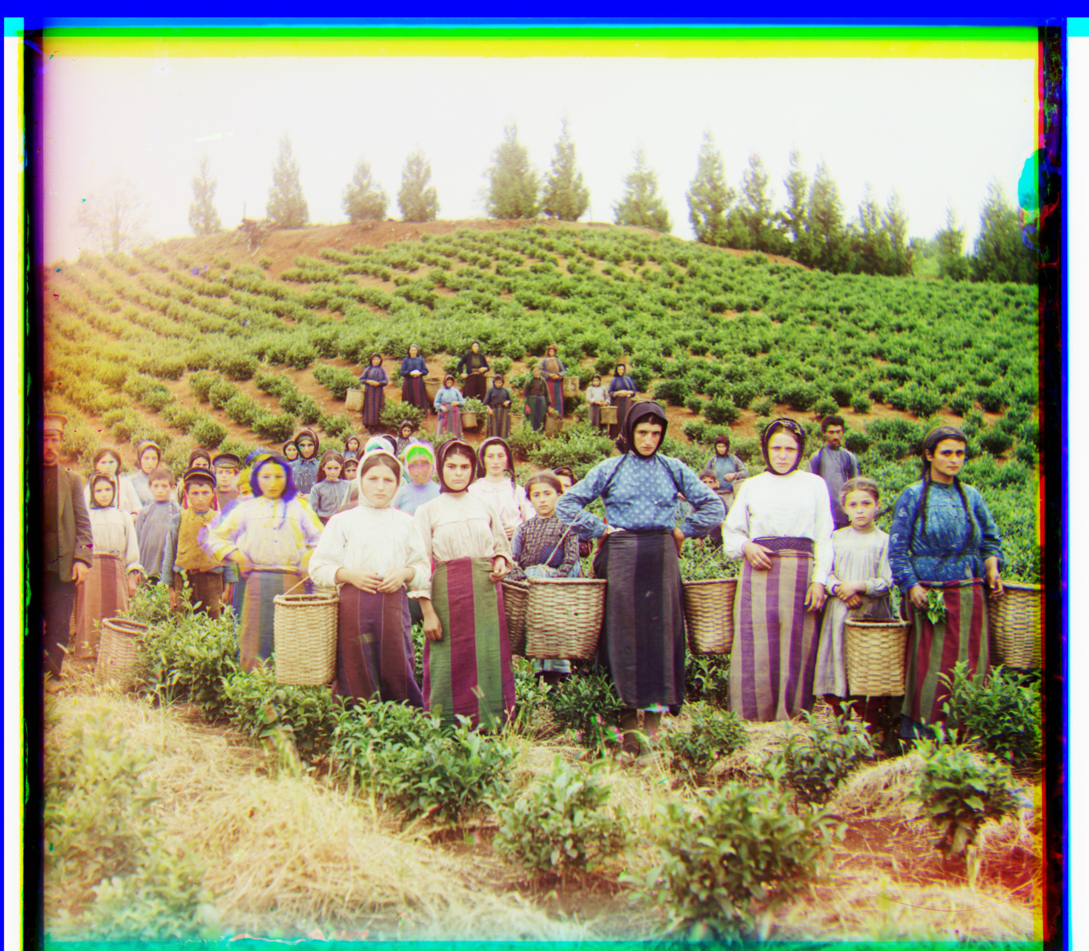
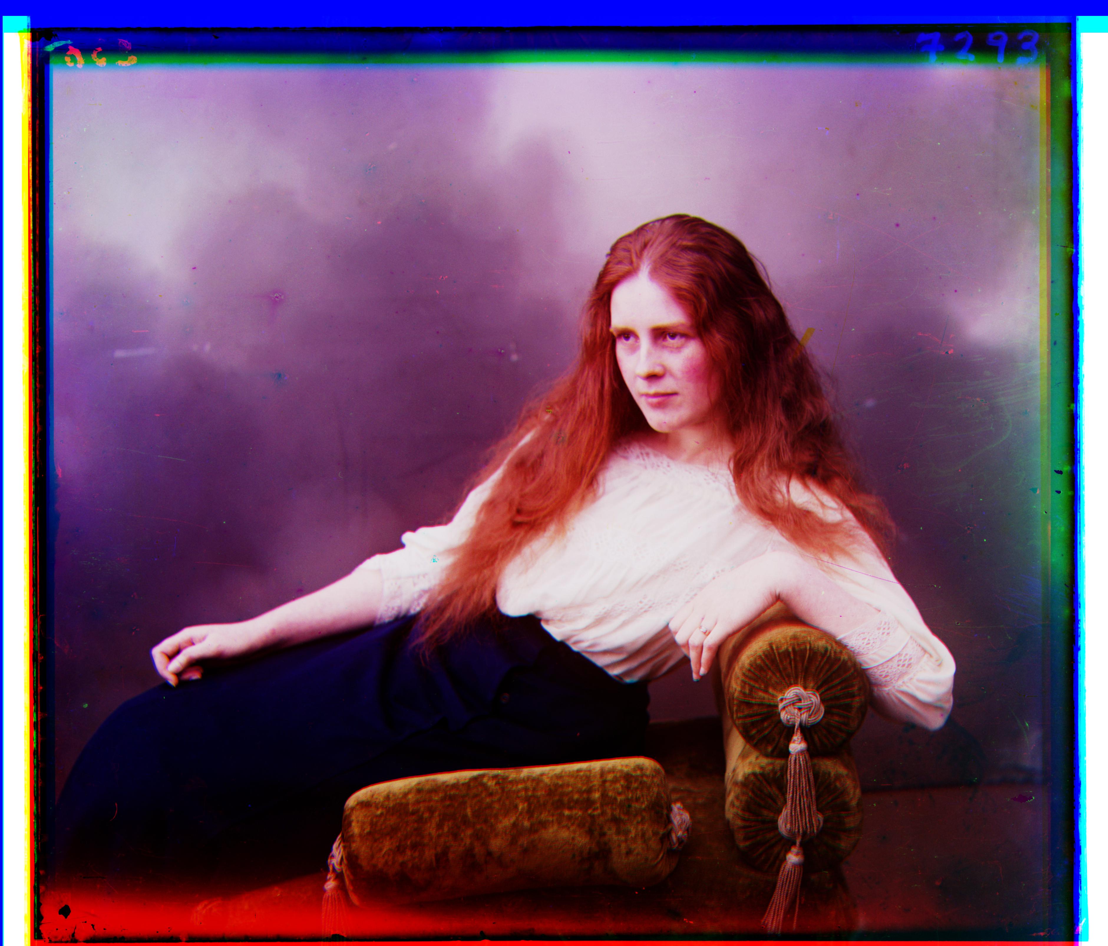
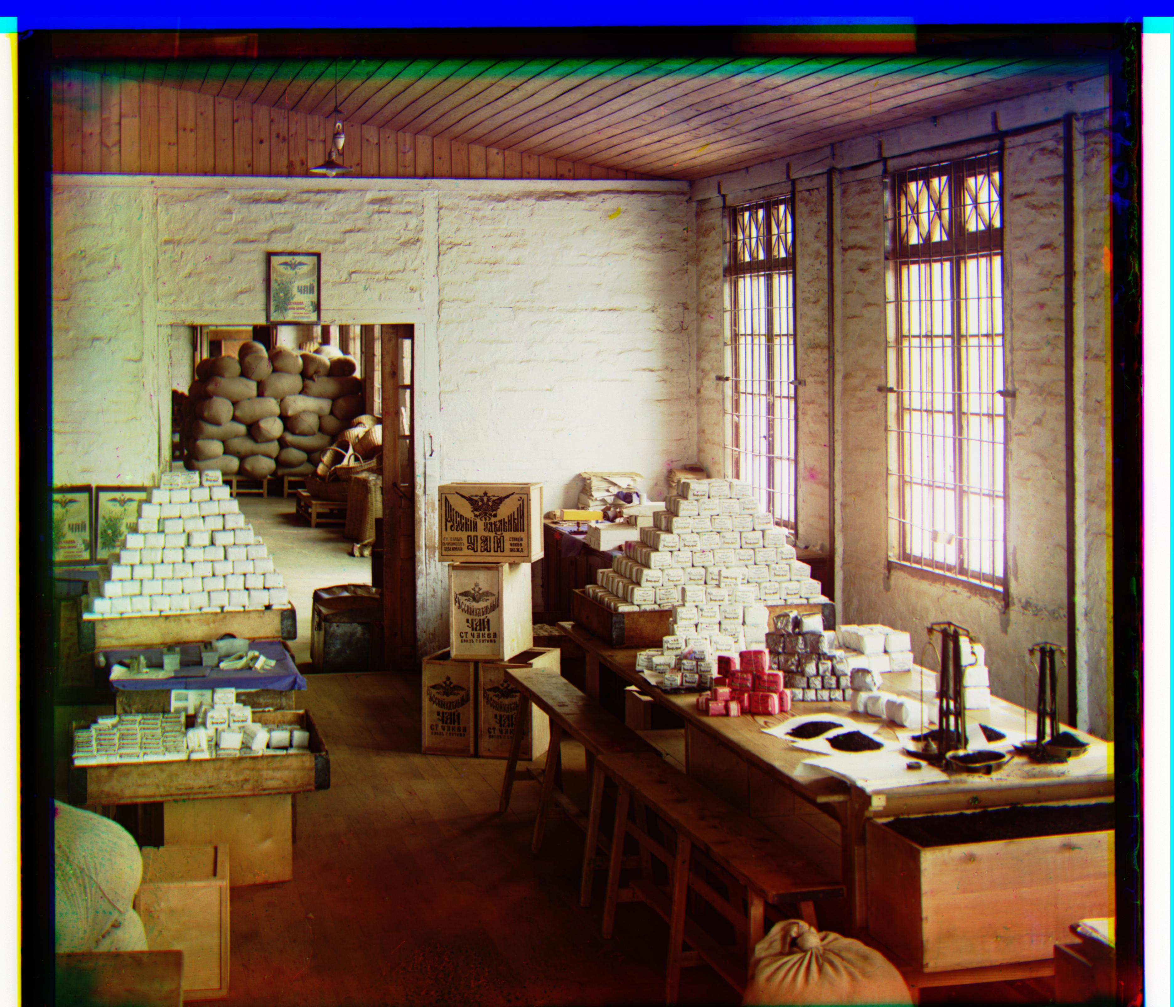
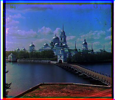
These are more reconstructed images from the photo collection that use the edge features, but no auto-contrast.
|
|
|