 |
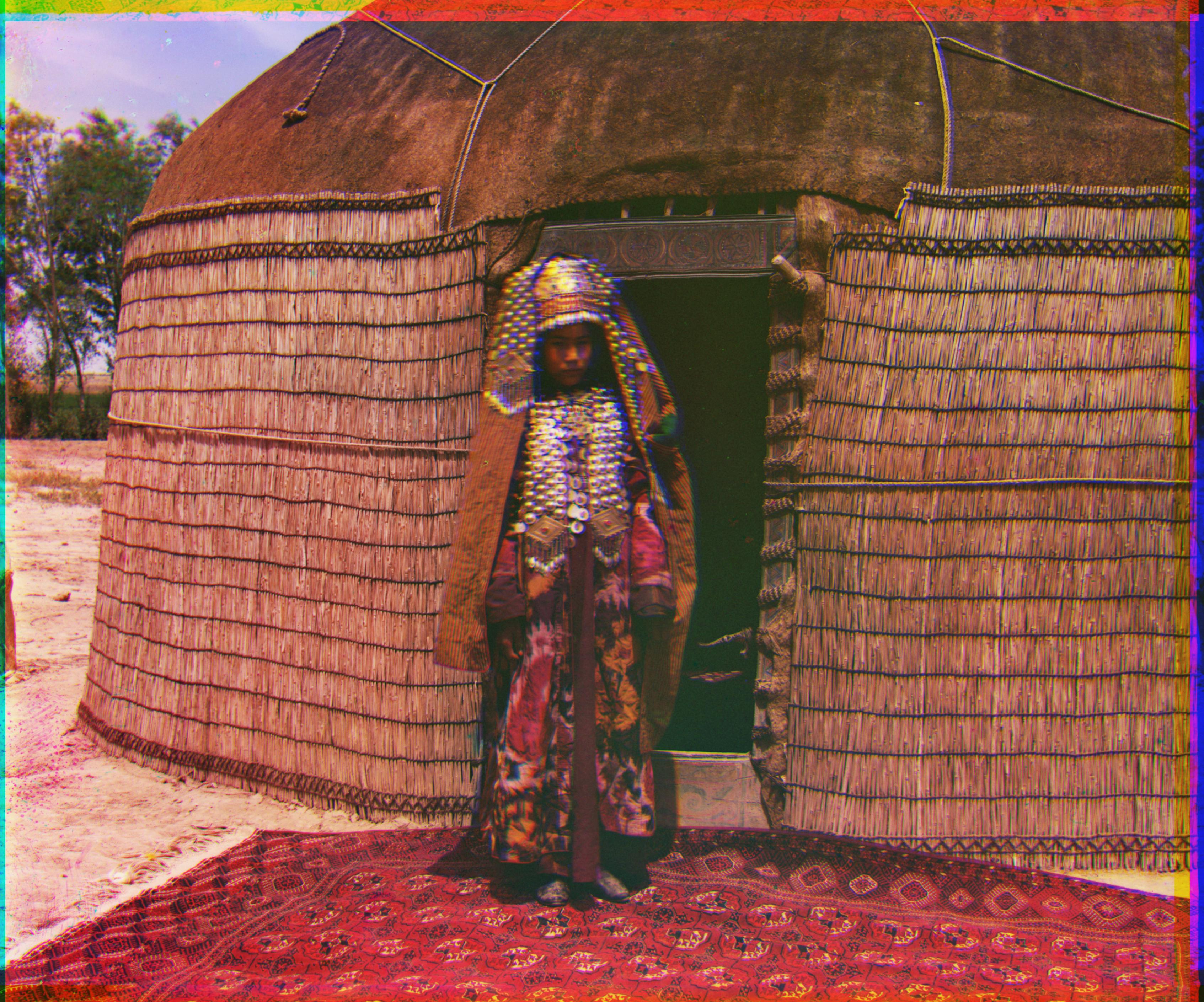
During the Russian empire, when colored photos did not exist, Sergei Mikhailovich Prokudin-Gorskii started to record all the scenes in Russia on a glass plate using red, green, and blue filter at 1907. Now, as the technology advanced, we can combine the three images to create a fully colored image.
In this project, I implement two functionalities, "Exhaustive Search" and "Image Pyramid", to restore the black and white images taken by Prokudin-Gorskii into color image.
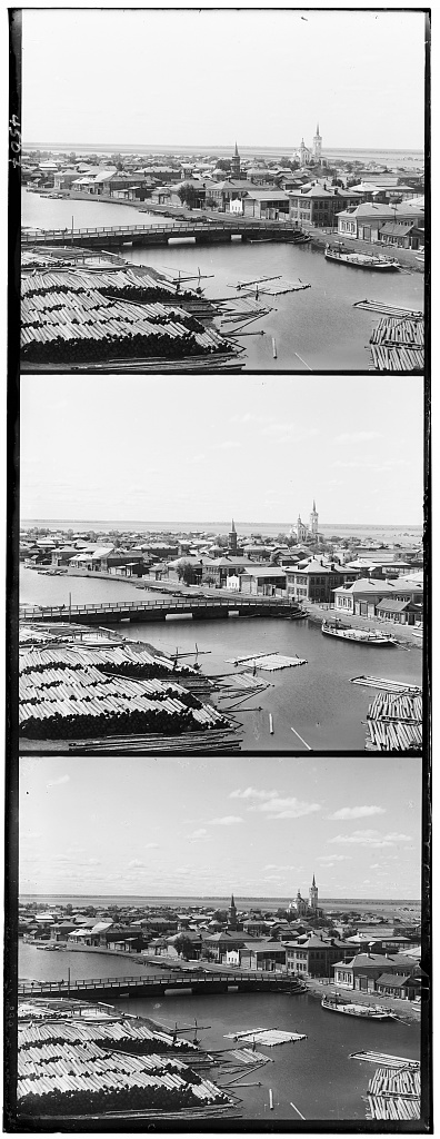
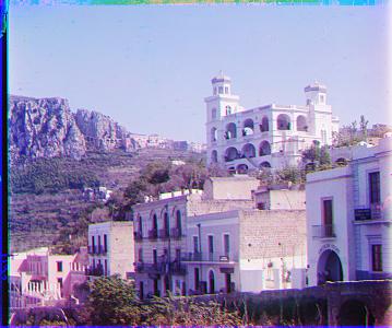
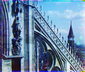
Input images for this project have forms of the following:
|
|
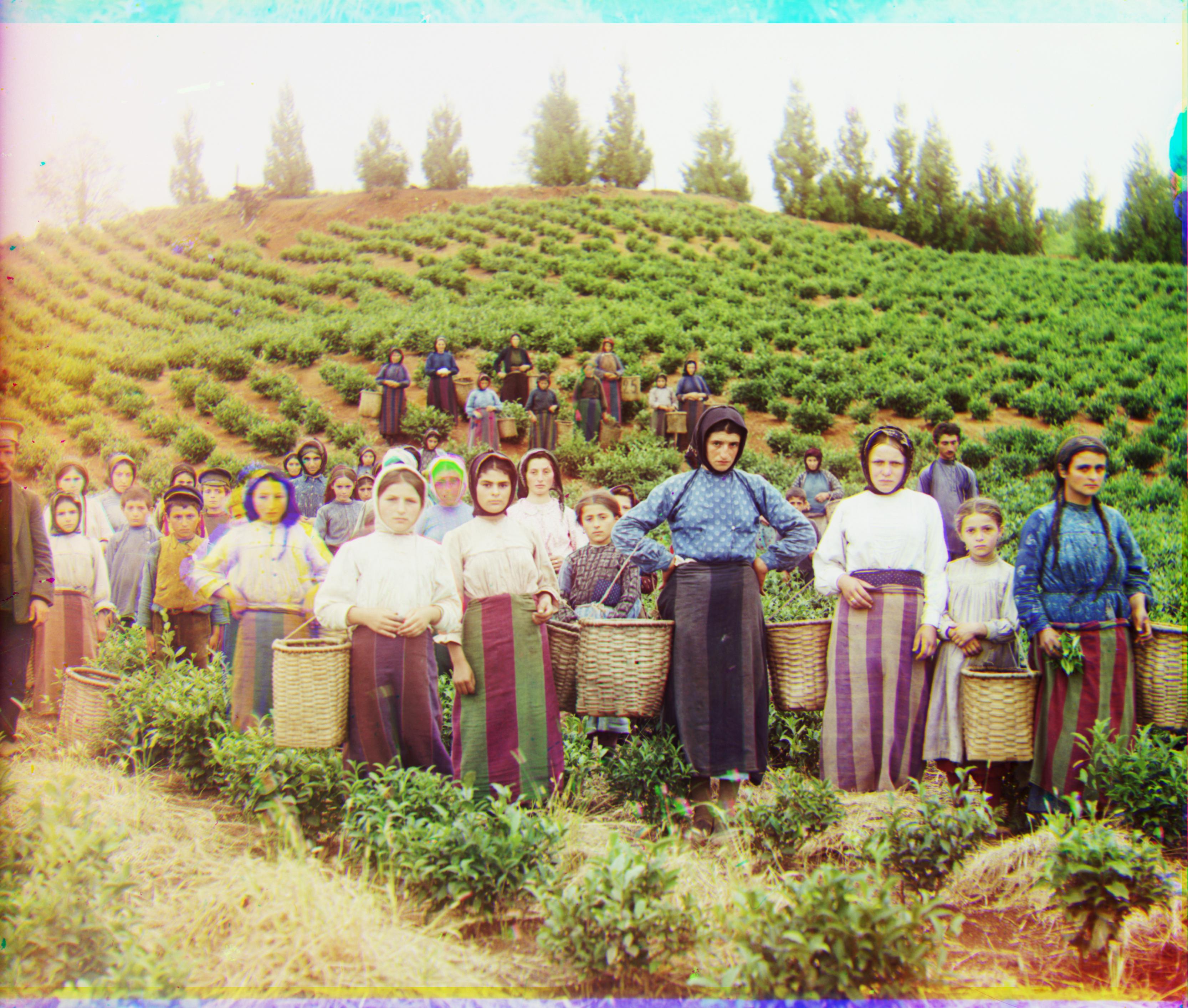
Three photo scenes from above are each taken with blue, green, and red filters, and the goal of this project is to align those three images as perfect as possible to create a well aligned colored image. In order to have as much accuracy as possible for this project, I cropped out the border lines and divide the image into 3 sections having exactly identical width and height.
As images taken from each filter is not well aligned, I pick the image taken with green filter to be the reference and displace images taken by blue and red filters to align well. And there are two key aspects on achieving this task:
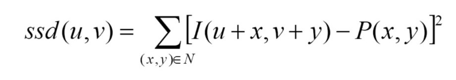 |
 Red Offset: (0, 7) |
 Red Offset: (0, 6) |
 Red Offset: (0, 4) |
 Red Offset: (0, 5) |
 Red Offset: (0, 7) |
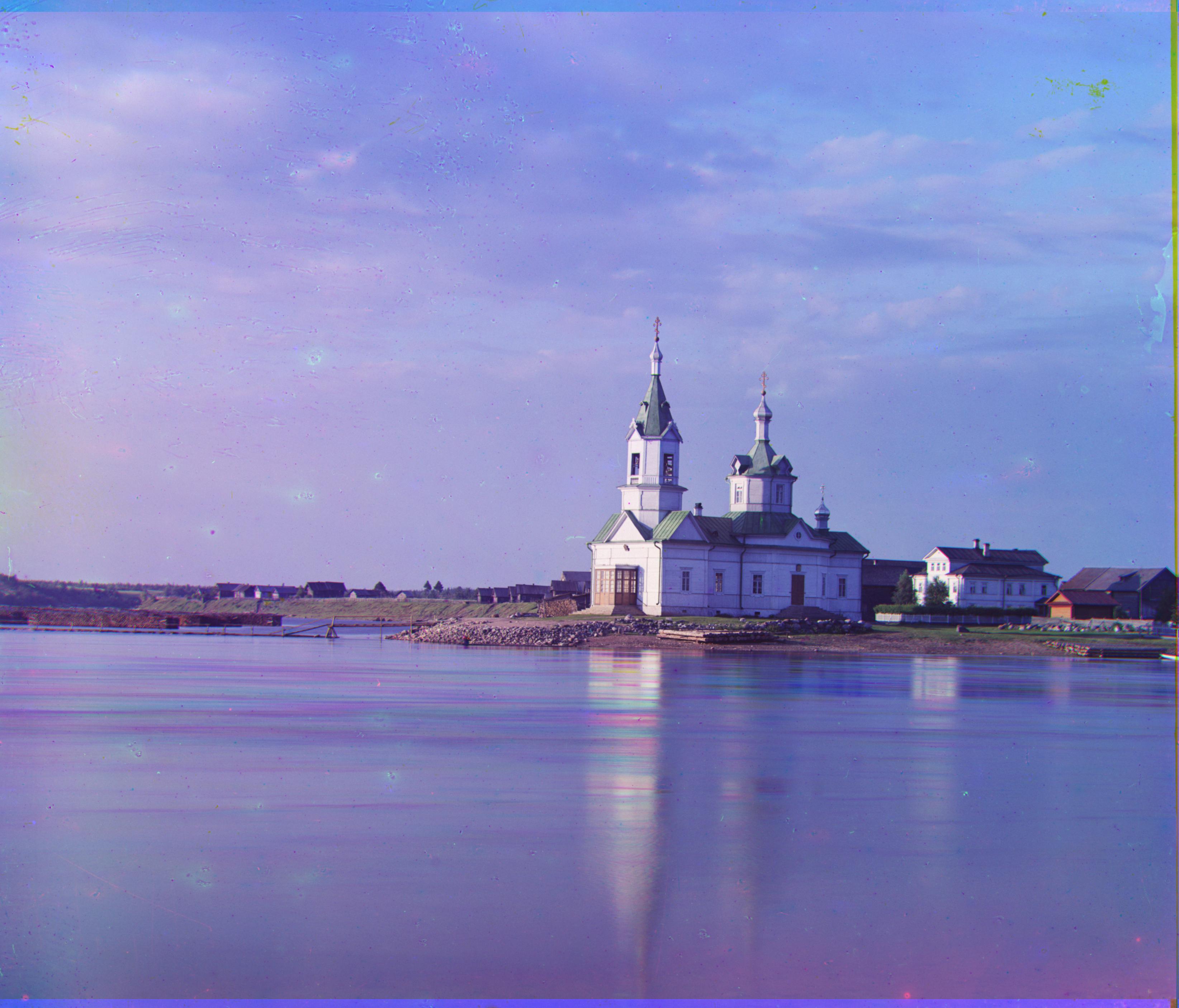
Simple exhaustive search were good enough for the low resolution images like .jpg. However, If the image size gets much bigger, like .tif, it can take very long time to find the best displacement as the number of pixels it has to search through increases as well when the size of the image increases. And implementing Image Pyramid can reduce this time to find the best displacement for large image.
Image Pyramid basically reduces the scale of the image until its size becomes small enough to find the best displacement with exhaustive search in reasonable time. Say we rescale the image in 1/2 for attempt to rescale. When the scale of the image becomes reasonably small, we perform the exhaustive search on it to find the best displacement for the small image. Then, we multiply this displacements by 2, so it can correspond to the image before it was halved. With the replacement, given for the larger image, we start the exhaustive search from there and find the best displacement. And we repeat this process until we perform the exhaustive search on the original scale image. This can be easily implemented with recursive function.
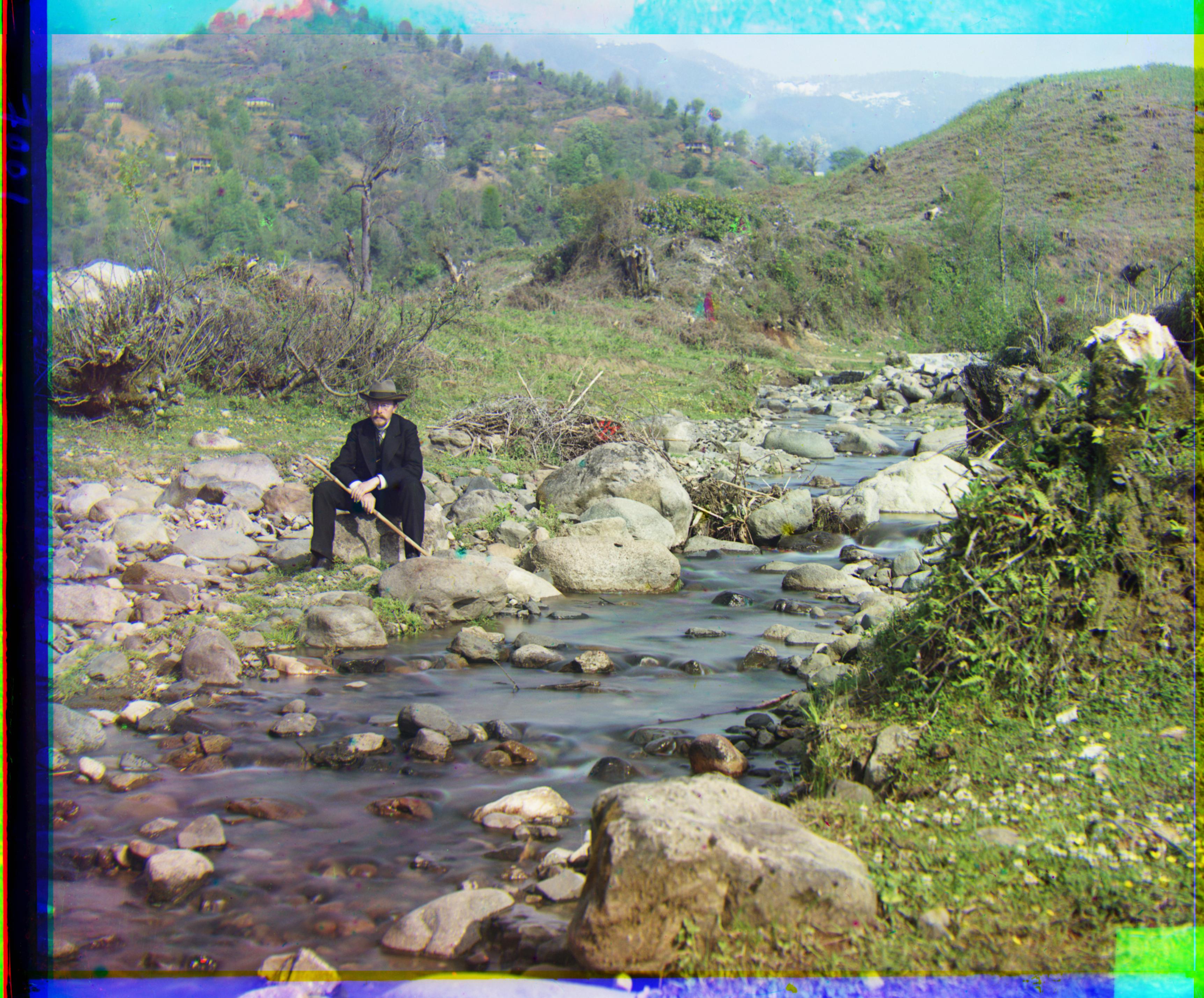
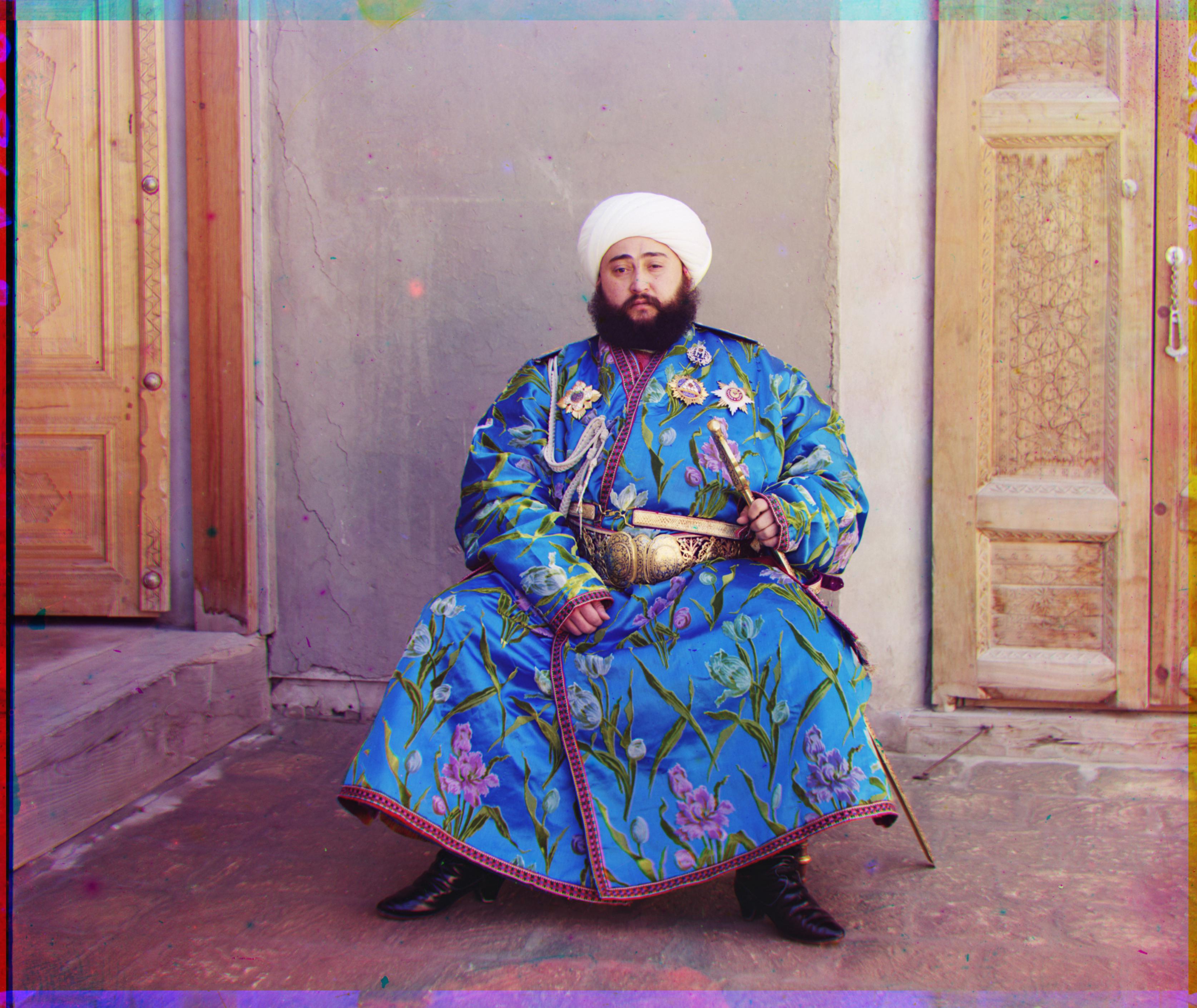 Red Offset: (17, 57) |
 Red Offset: (-8, 33) |
 Red Offset: (-3, 65) |
|
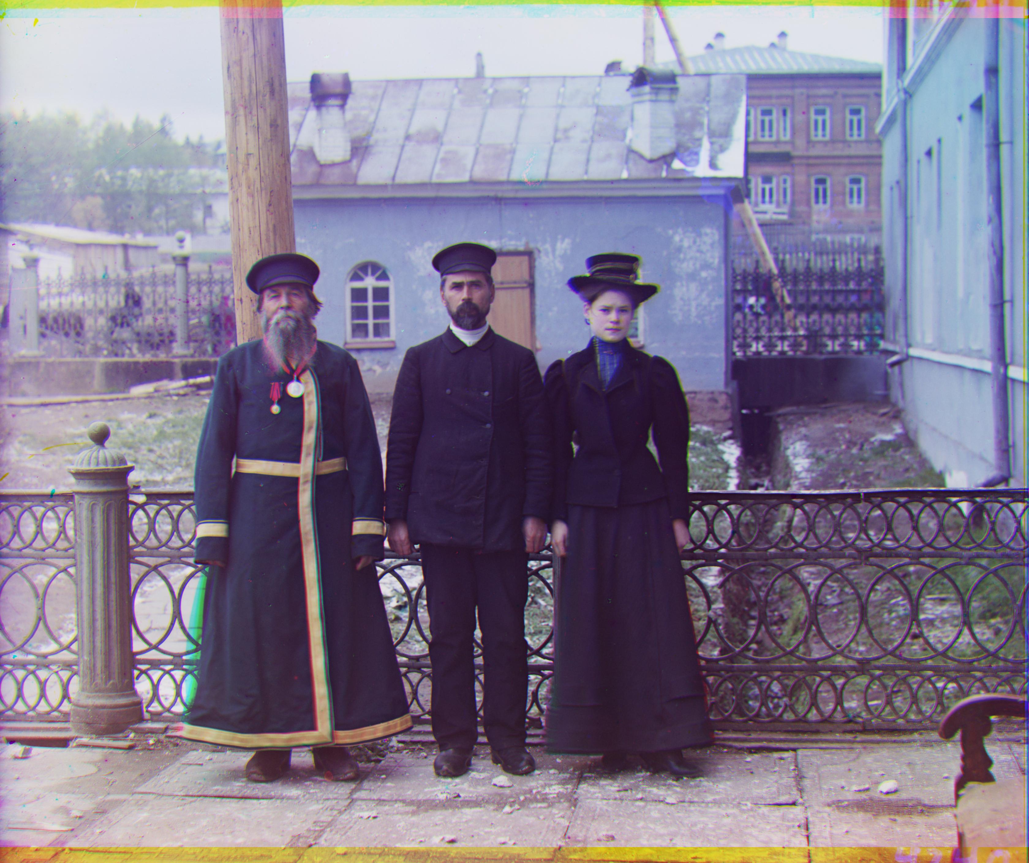
Red Offset: (5, 48) |
 Red Offset: (4, 60) |
 Red Offset: (3, 96) |
 Red Offset: (10, 57) |
 Red Offset: (8, 98) |
 Red Offset: (-2, 59) |
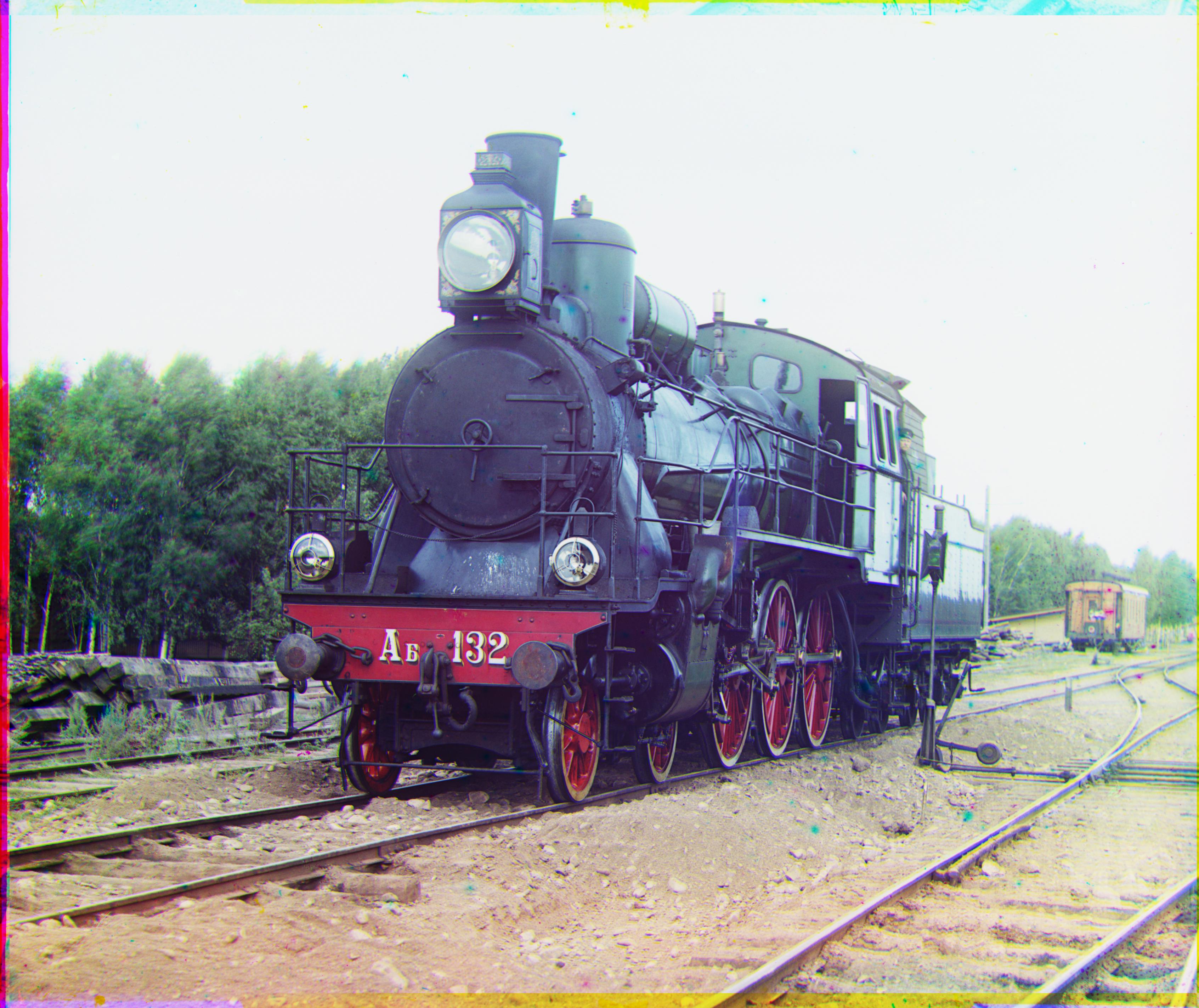 Red Offset: (27, 43) |
 Red Offset: (-11, 52) |
 Red Offset: (-43, 67) |
 Red Offset: (15, 60) |