COMPSCI 194-26: Project 1

Background

The Prokudin-Gorskii Collection

Sergei Mikhailovich Prokudin-Gorskii was a man well ahead of his time. Convinced, as early as 1907, that color photography was the wave of the future, he won Tzar's special permission to travel across the vast Russian Empire and take color photographs of everything he saw including the only color portrait of Leo Tolstoy. And he really photographed everything: people, buildings, landscapes, railroads, bridges... thousands of color pictures! His idea was simple: record three exposures of every scene onto a glass plate using a red, a green, and a blue filter. Never mind that there was no way to print color photographs until much later -- he envisioned special projectors to be installed in "multimedia" classrooms all across Russia where the children would be able to learn about their vast country. Alas, his plans never materialized: he left Russia in 1918, right after the revolution, never to return again. Luckily, his RGB glass plate negatives, capturing the last years of the Russian Empire, survived and were purchased in 1948 by the Library of Congress. The LoC has recently digitized the negatives and made them available on-line. In this project, I attempt to combine these seemingly black and white images with different color filters, into a single colored image.

Naive Exhaustive Search using Similarity Metrics

A simple stacking of the 3 channels is not good enough because each channel is slightly different, due to either the environment changing ever so slightly, or just the camera moving between different clicks. So before we can stack the channels, we must try to align them. To do this, I tried two different similarity metrics: Sum of Squared Differences (SSD) and normalized cross-correlation (NCC). SSD is the L2 norm of the difference of 2 channels, where a higher score represents a greater difference between images. So lower scores are better. NCC is the dot product between two normalized vectors. To convert 2D images into vectors, I flattened them and then compared them. Since they are normalized vectors, a perfect match would have a dot product of 1, and the score gets closer to 0 as the images get more and more different. So a higher score is best. To find the best alignment, I used an exhaustive search over a range of [-20, 20] pixels in both the x and y direction. Based on my testing, I found that NCC performed significantly better than SSD. So for all (small) images, I ran SSD with exhaustive search.

Cropping

The borders of each of the channels are slightly chaotic and don’t line up well. Using these values would make our similarity metric return haywire results. So before we do anything, I cropped off 15% of the image on all 4 sides. This gets rid of the noisy borders, and only uses good, reliable, internal pixels. In addition, when translating a channel, part of the image is filled with 0s. This made NCC give strange results. I started with a color image, split it into 3 images, and translated the R channel by (10, 10) followed by (-10, -10). In theory, ncc should return a perfect match. But it didn’t, and even thought a non (0,0) translation gave better results. So whenever I translated an image, I cropped out the amount by which it was translated to ensure there are no extra 0s. As I write this report, I realize I could have used np.roll to roll the borders to the other side, instead of the WarpAffine shown at the python tutorial. While this wouldn’t have changed the results by much, it should save some time by not having to crop part of the image every time it is translated (done 1600 times for an exhaustive search over [-20, 20]

Exhasutive Results on JPEG images

Here are some results on smaller (.jpeg) images:

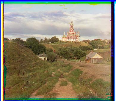
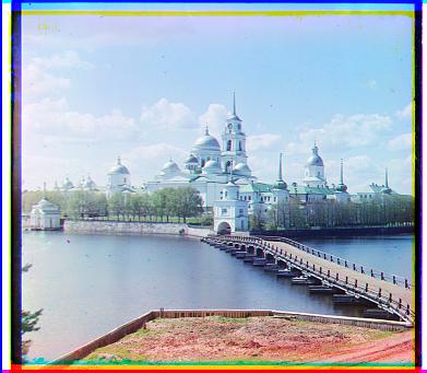
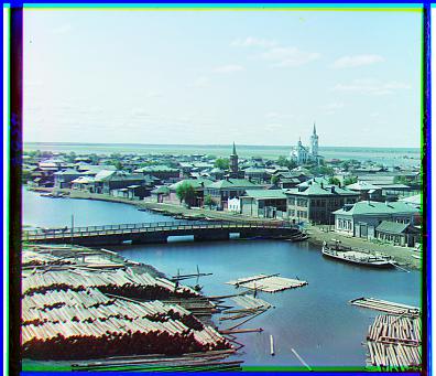
Image Pyramids to speed up search on bigger images

On bigger images, this technique doesn’t work as well because we expect bigger translations than a max of 20 in x or y. Increasing the range beyond [-20, 20] makes exhaustive search extremely slow as it searches every x,y combination, resulting in x*y runs. To speed this process up, I used a coarse-to-fine image pyramid. An image pyramid contains the original, high quality image at the base of the pyramid, and then as you work your way up, the image is rescaled to be smaller than before. So at the top of the pyramid, is the coarsest, lowest quality image. We first run the original exhaustive search on the coarsest image to get an initial estimate of the translation needed to align the image. We then work our way down the pyramid, only trying translations near the one returned by the level above. If the layer above us returned a translation of (50, 50), we know that there’s no point trying translations like (-75, -40) which our original exhaustive search would have done. So we can just focus on translations around (50, 50), and we save a lot of time in this way.

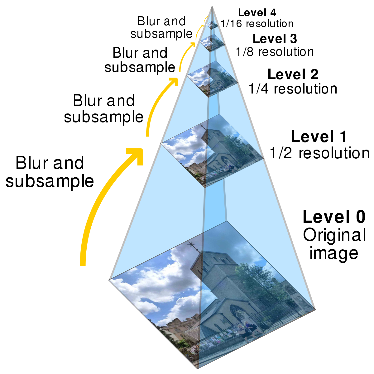
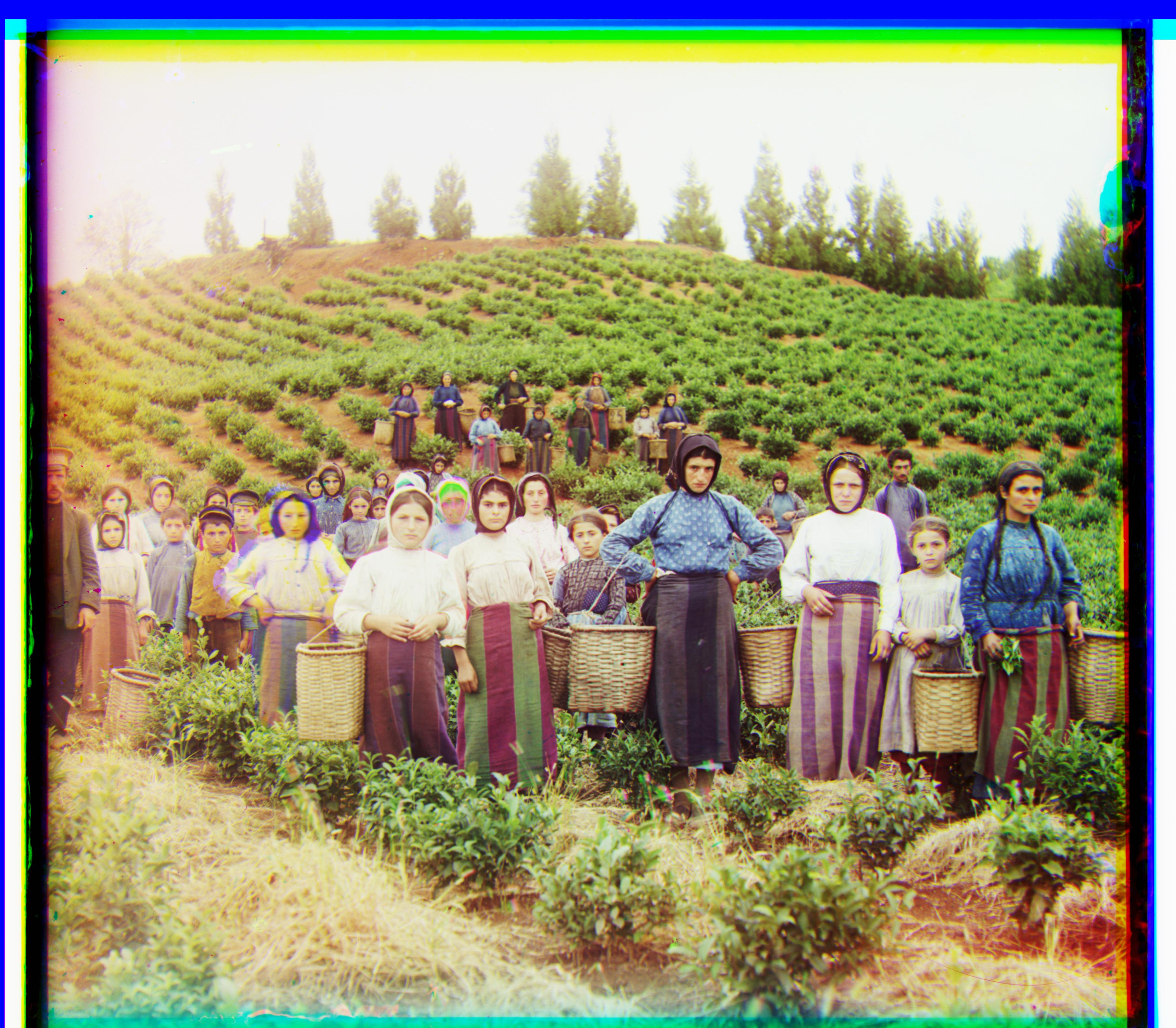
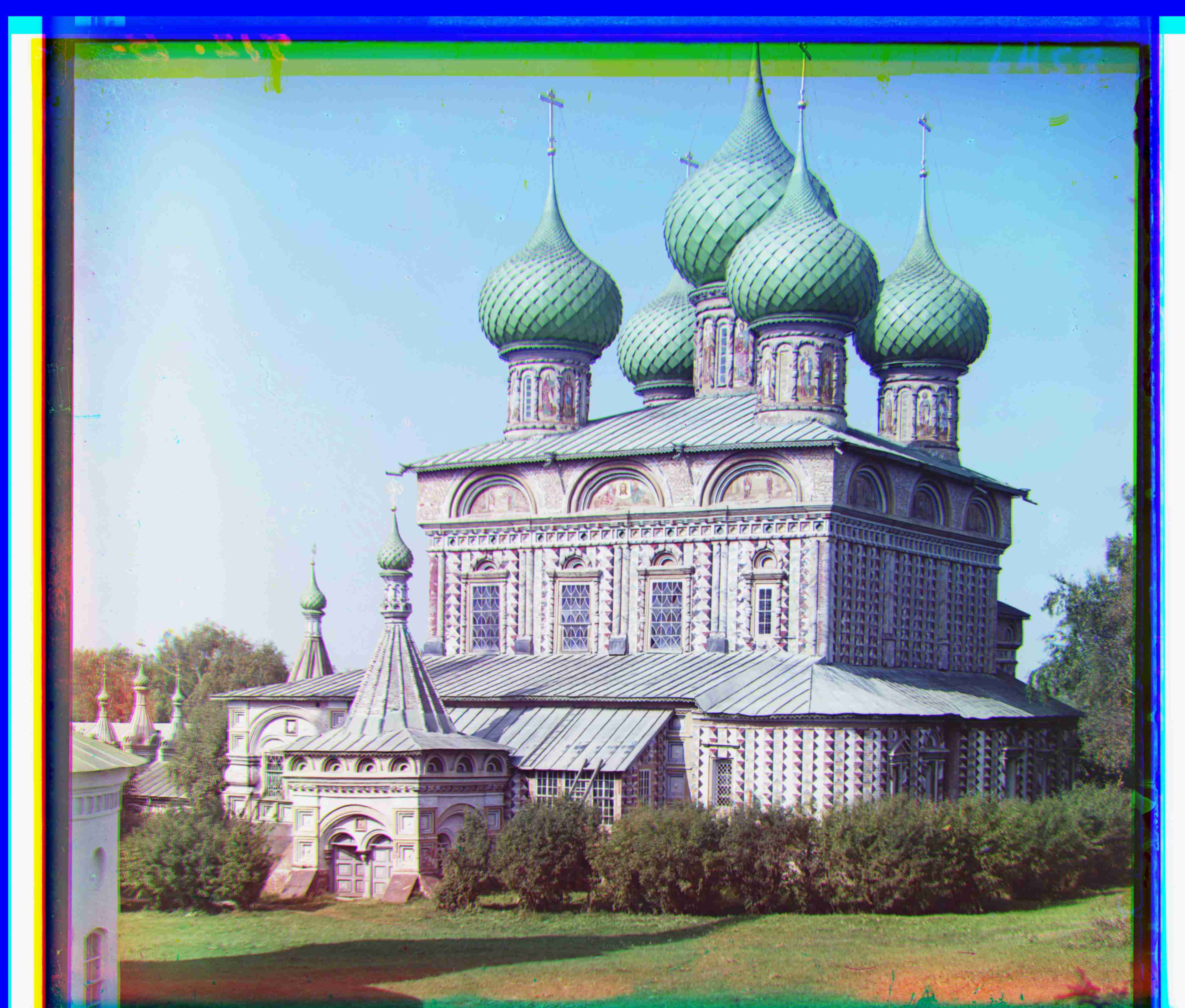
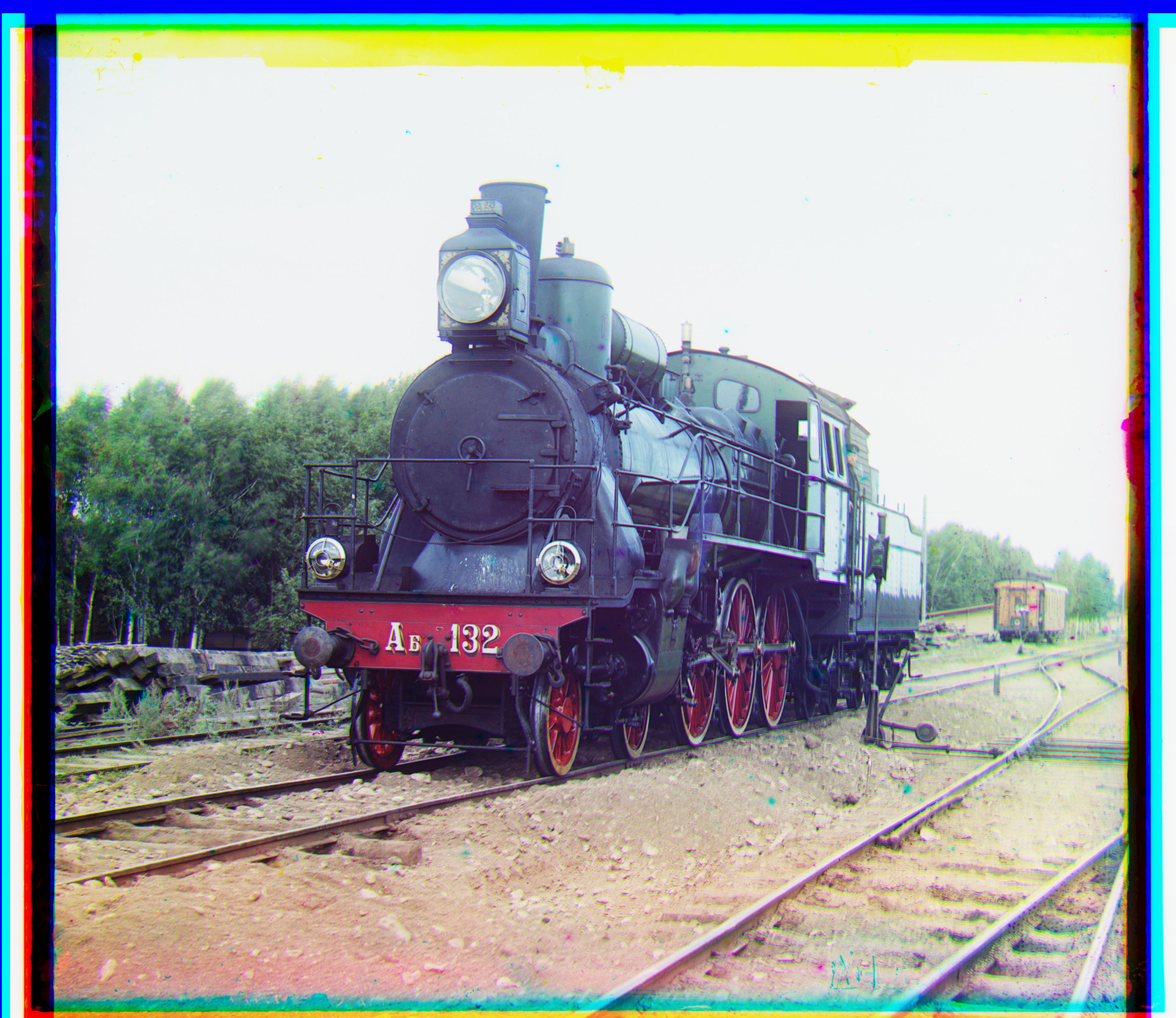
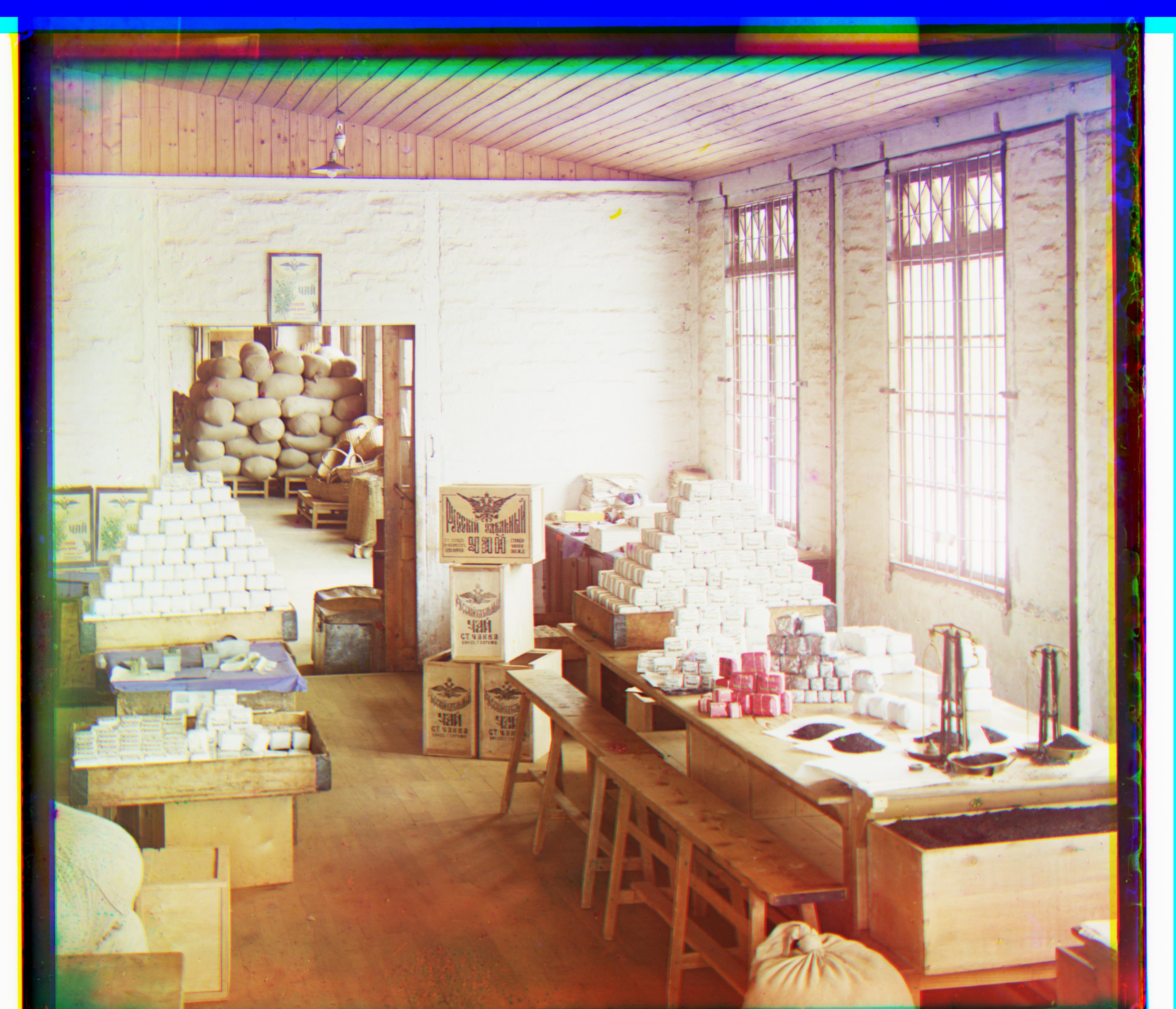
Image Pyramid Results on TIFF images

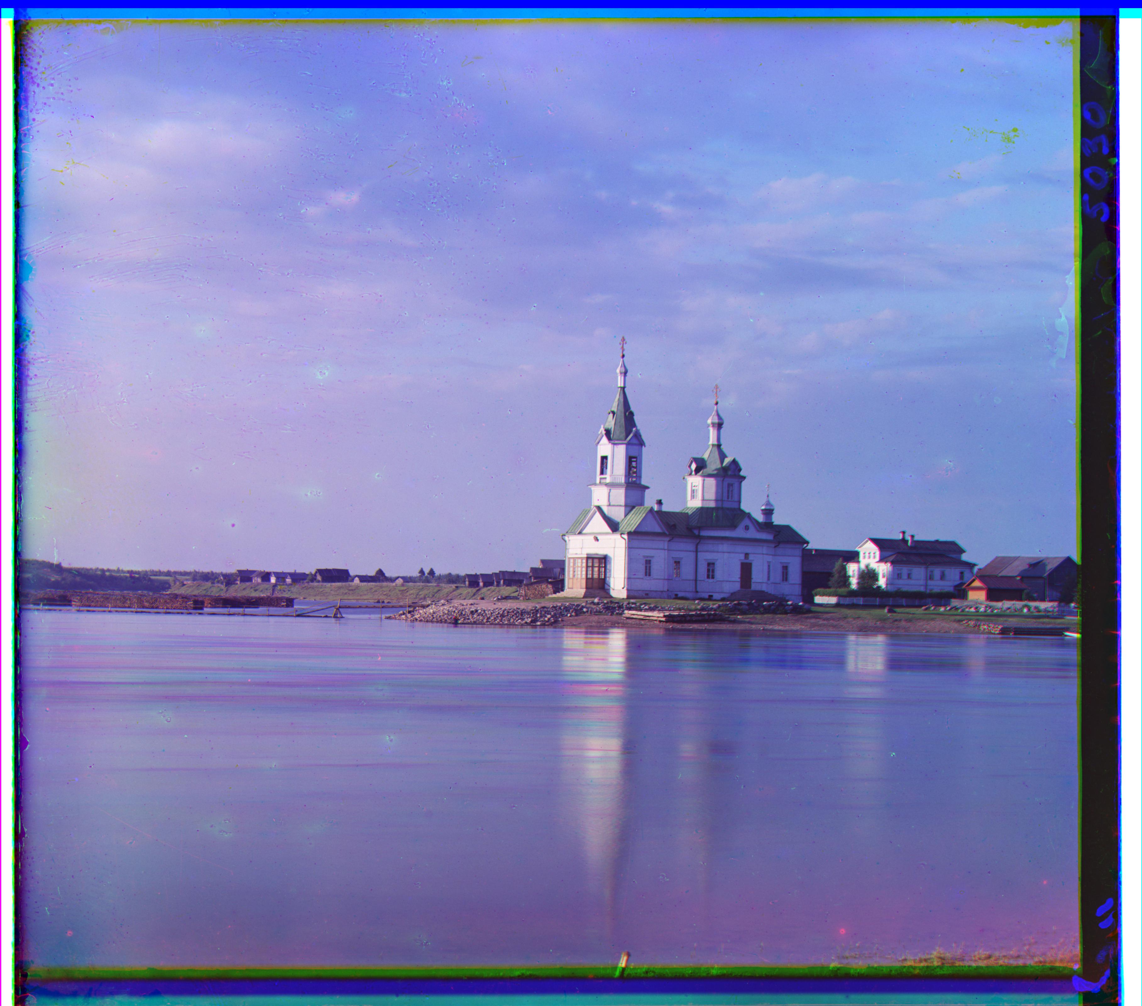
Here are some results on big (.tif) images:

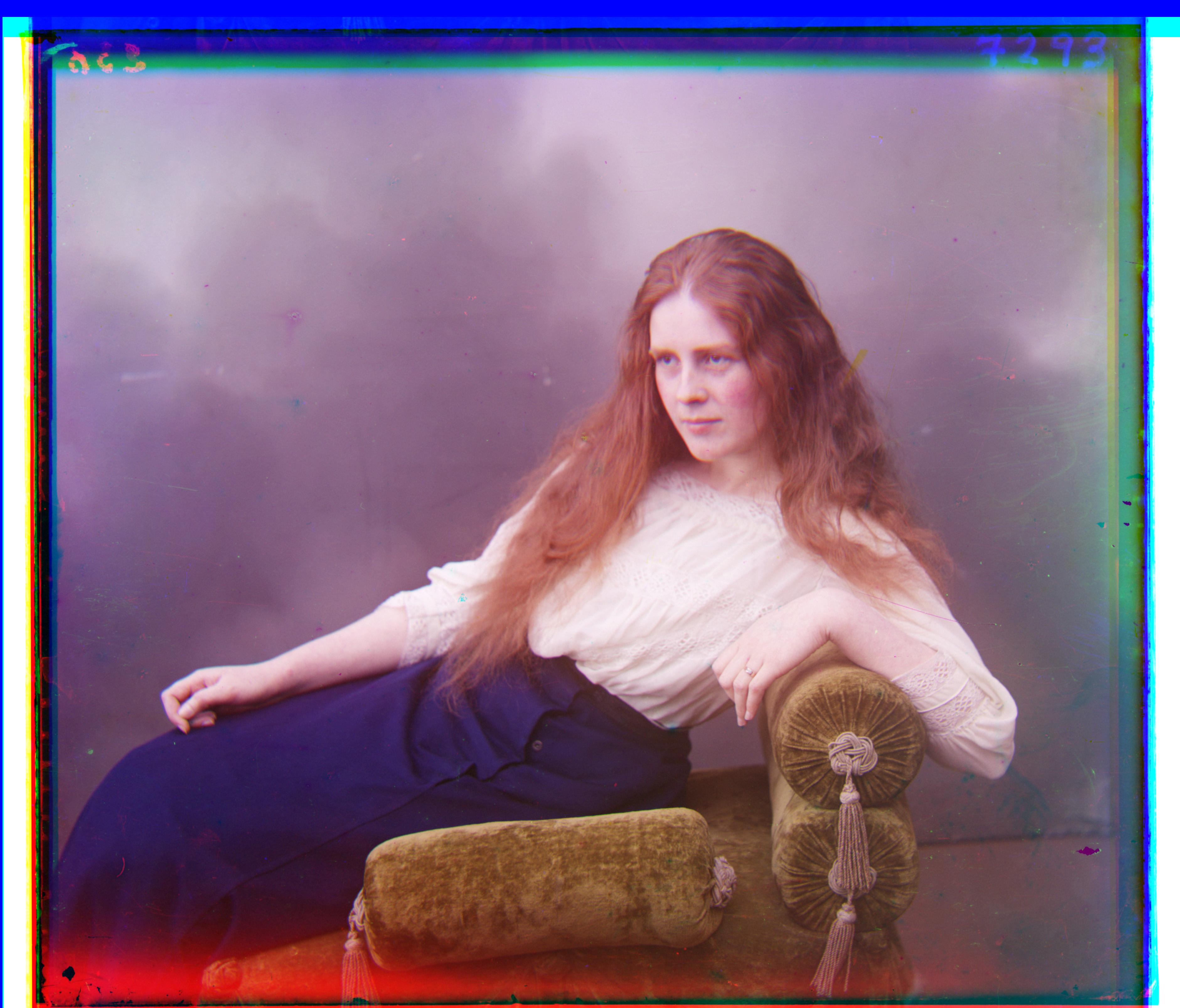
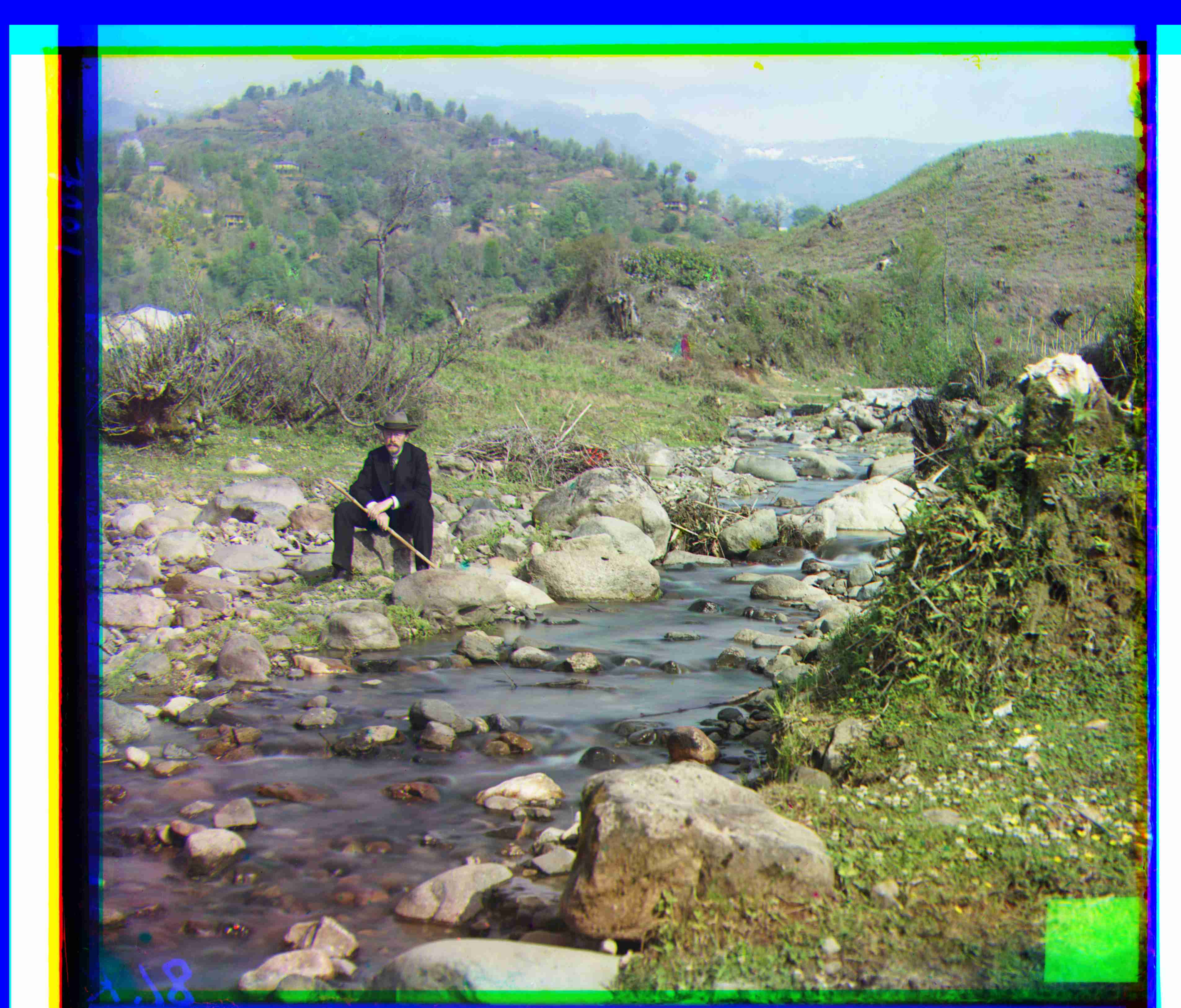
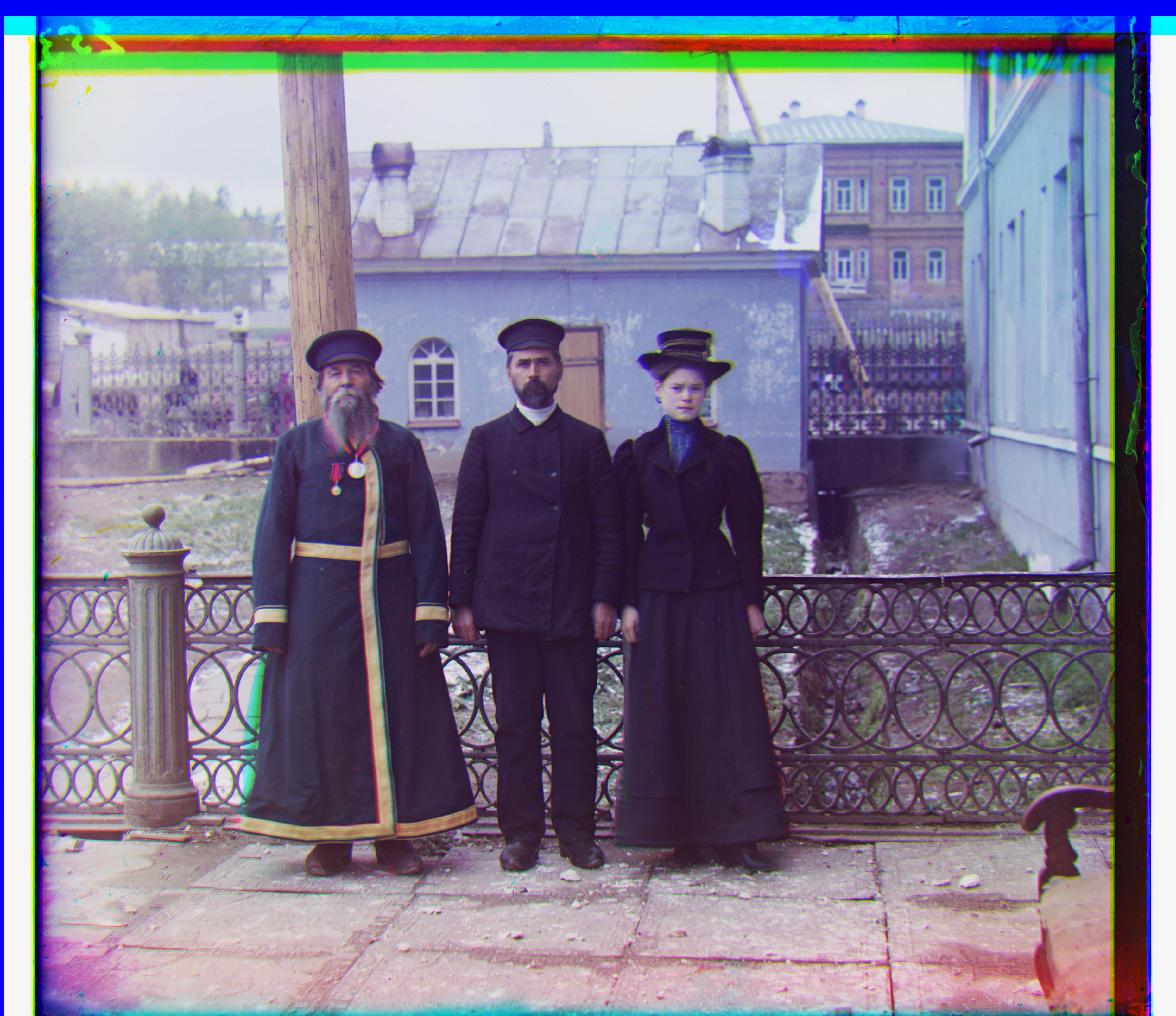
Additional Results

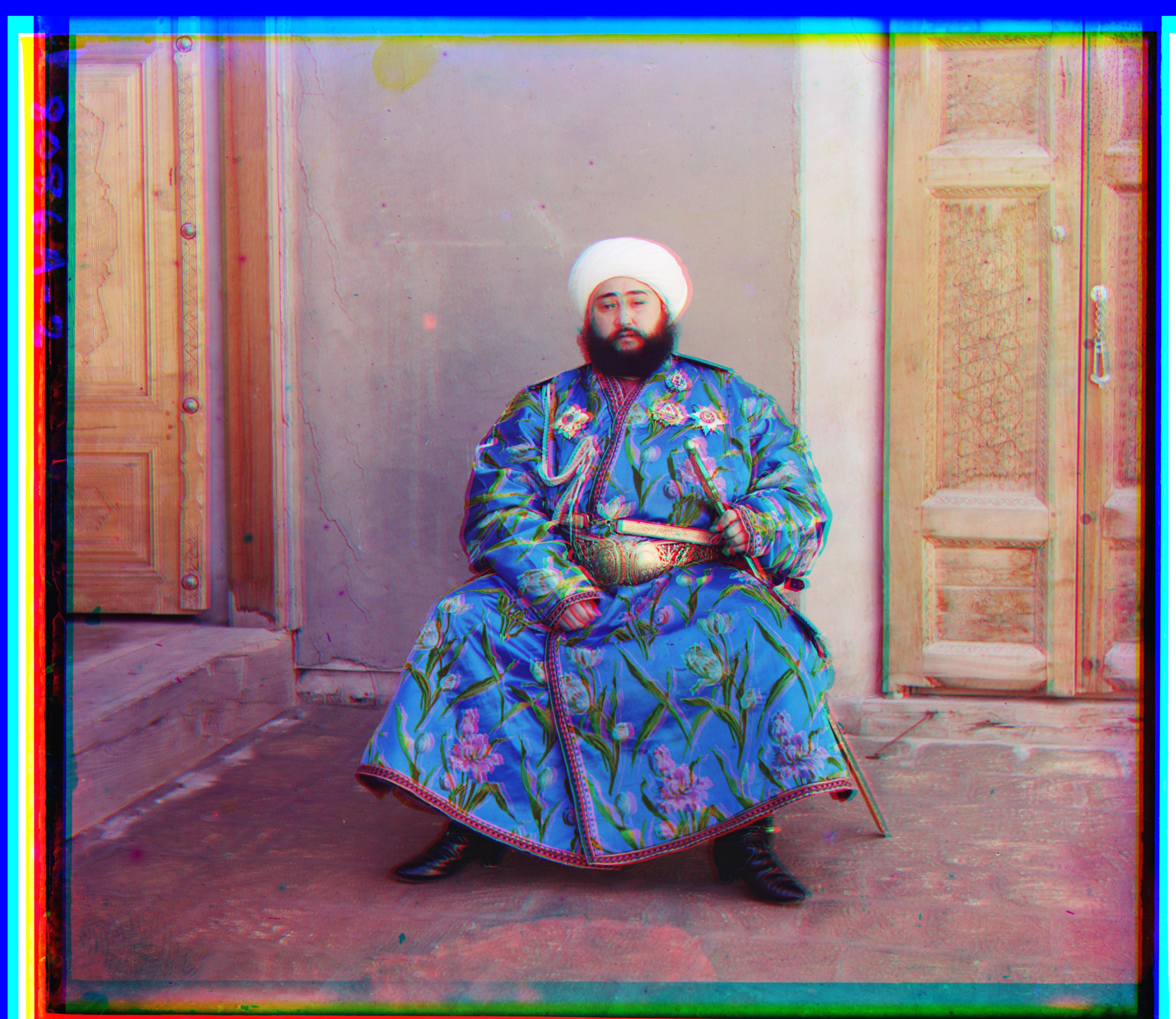
Here are some results on images outside of those given in the .data folder of the project spec (these images can be found here):

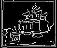
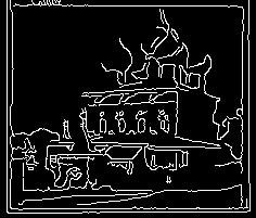
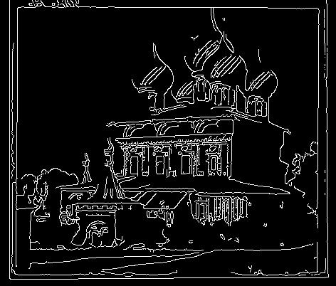
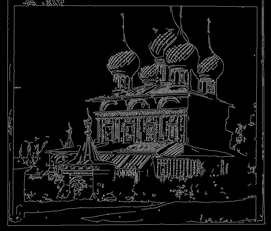
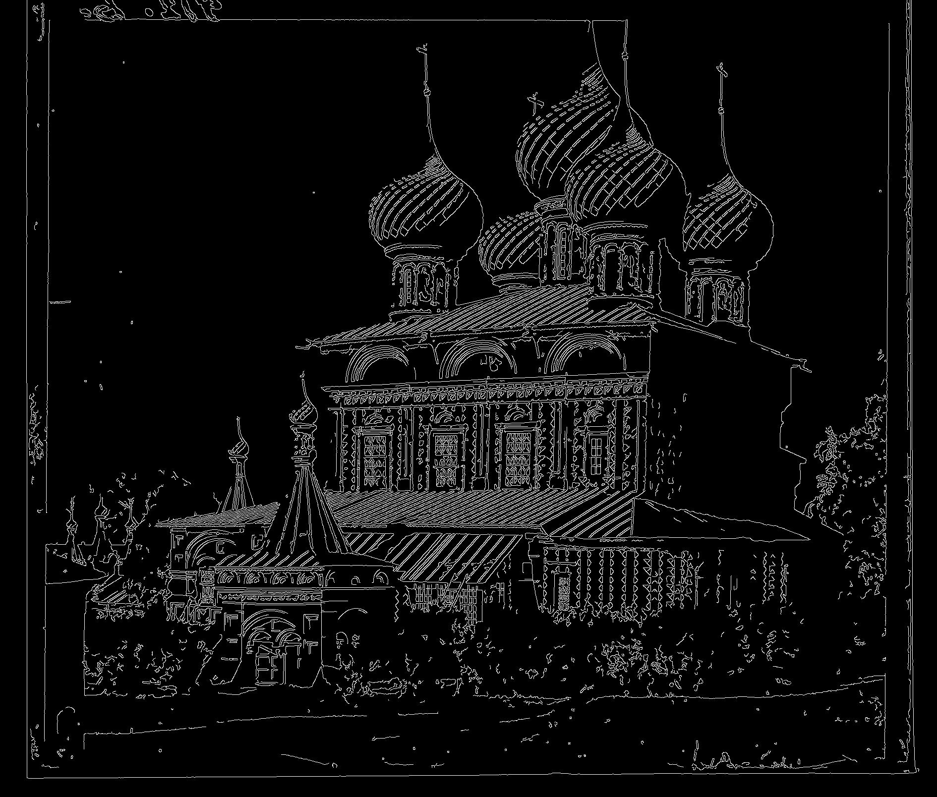
Edge Detection

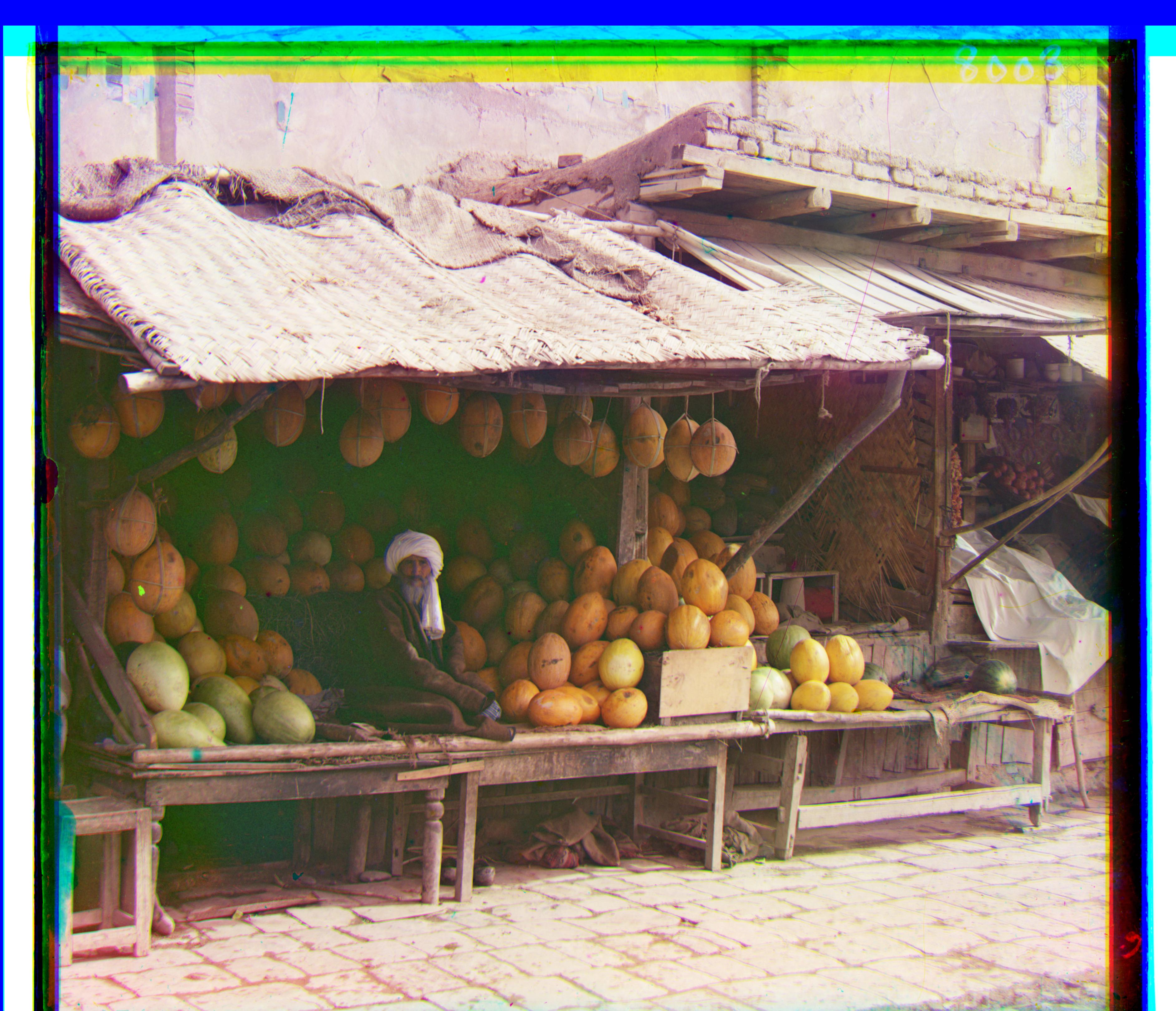
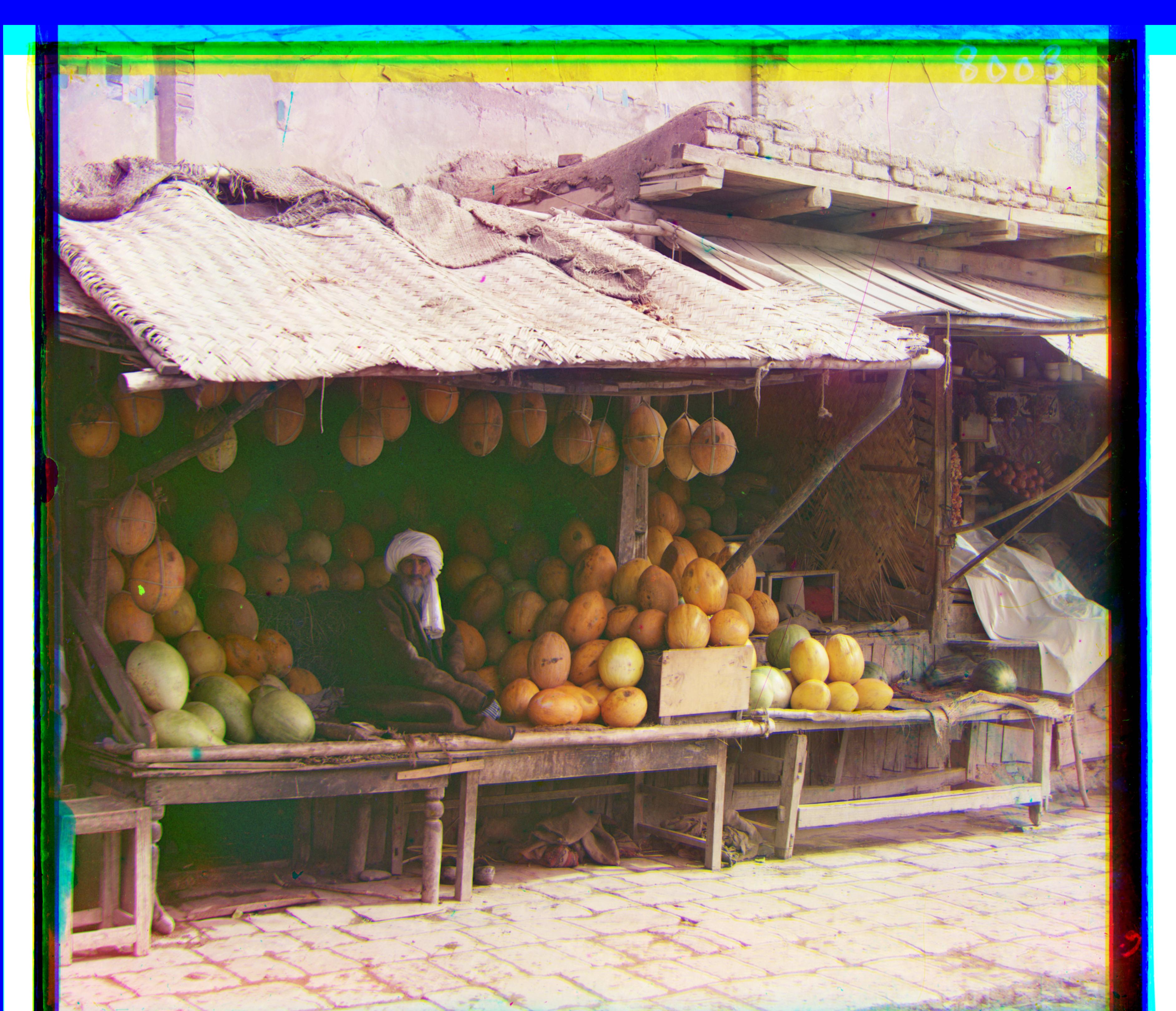
For the main assignment, we used the raw pixel values of each channel. However, this isn’t the best metric because pixel values don’t need to be the same across different channels. In fact, if they were, the 3 channel stacked image would be grayscale. A better metric to align images is to first find the edges in the image (which tell a simpler story about the image), and then lining up 2 images with only edges. I used Canny edge detection, and here are some results: Using edges worked best with SSD over NCC, and was a bit faster than the naive NCC alignment. For the regular image pyramid, due to time restrictions, I had to use the values from the 2nd from the bottom layer (not the bottom-most = finest layer), so the final translation wasn't based off of the highest quality image. With edge detection and SSD, it ran fast enough that I could go all the way to the bottom. This adds some minor accuracy to the pictures we use, and is expected to add much more accuracy to bigger pictures where naive NCC might be too slow. Here is an example of melons.tif, using naive NCC versus edge detection with SSD. The difference is not visible, but there is a couple pixel difference due to the extra run on the highest quality layer of the image pyramid.

And here, we can see the effect of using edge detection on our image pyramid. Instead of comparing background pixels and other noisy information, we are only comparing the most important information (and what I use as reference when determining whether the image is actually aligned). This means our similarity metric (SSD in my case) is only affected by important pixels. This also helps us visualize the usefulness of the image pyramid. In the first image, we can just kind of tell whats going on, and in each next layer, we get more and more information. But even the coarser images are good enough to get a decent estimate of how to align an image.