Sergey Prokudin-Gorskii was a pioneer in photography who is known for his photogaphic documentation of Russia in the early 20th century. Prokudin-Gorskii's photographic style was different however, as he used a red, green, and blue filter to record three seperate exposures (or negatives) on glass at once. Even though his grand plans of travelling Russia to document her was cut short and many of his works/pieces have not been found, the Library of Congress was able t0 digitize a few of these negatives and release them for free on the internet. A naive way to colorize these digitized images would be to split them in thirds for each color channel (r, g, b) and stack them on top of each other. However, this often is suboptimal since the filters obtained after splitting the negative into thirds are often not perfectly aligned. Thus, this project worked on finding the necessary translations/offsets for 2 of the filters such that all 3 are aligned post-stacking.
For images that are small enough, the single-scale (or exhaustive) approach was used. The approach takes two images of the same size and chooses the first image as the one it will be translating around. For example, when an image is translated by (4, -3) that means the rows have been translated/offset down by 4 and the columns have been translated/offset left by 3. In my single-scale implementation, the row and column offset were both searched for within the range [-25, 25]. For each (row offset, column offset) tuple, the SSD (sum of squared differences) is found between the offsetted image1 and image2. More specifically, only the middle square, which is defined as a square of size 2 * min(image1.shape[0] // 3, image1.shape[1] // 3) centered on the image, of both offsetted image1 and image2 are used for the SSD calculation. The (row offset, column offset) tuple which minimized the SSD is then outputted as the optimal x,y / row,column offset.
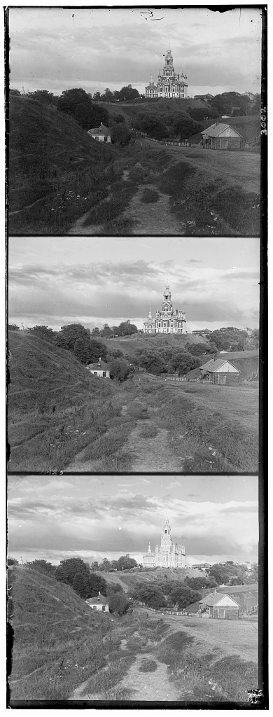
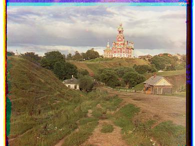
For the few small images I colorized using the single-scale implemenation, I have displayed the digitized negatives and the correctly aligned colorized output. I also have printed out the particular offsets that were found. All of these single-scale results are with using the blue filter as the base.
red offset = (12, 3), green offset = (5, 2)
red offset = (3, 2), green offset = (-3, 2)
red offset = (7, 3), green offset = (3, 3)
When images are too large, the small-scale implementation is too slow. Thus, another implementation had to be created for larger images. This multi-scale implementation will downsample large images (which are at the bottom of our "image pyramid") by a factor of 2 until the image is "small enough" (which will be the top of our "image pyramid", such as smaller than 400 * 400 in my case. At that point, the small-scale implementation is run and the optimal offsets are calculated for the smallest/most downsampled image/top of our image pyramid. Now we must traverse back down the image pyramid until we are at our original, large image. When we traverse down the image pyramid, we must scale our previously calculated offsets by a factor of 2 and use the newly scaled offset as the starting point for our current level. Let me explain with an example. Let's say we have an image which is 600 x 600. So we downsample to get a 300 x 300 image. Let's say the optimal offset was found to be (-3, 9). That is the optimal offset for the top of the pyramid. We must come back down. When we come back down a level to our original level, the offset of (-3, 9) becomes (-6, 18) and we will search [6 - 15, 6 + 15] and [18 - 15, 18 + 15] for our x and y offsets, respectively.
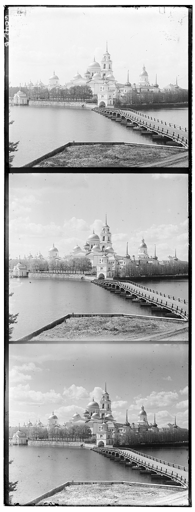
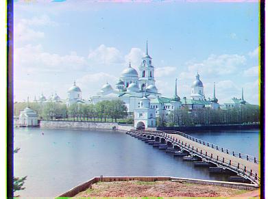
I displayed correctly aligned colorized output and printed out the resultantoffsets that were found. All of these results are with using the blue filter as the bas (unless specifically said otherwise). On average, the amount of time these images took to colorize was about 30-50 seconds.
red offset = (114, 12), green offset = (53, 8)
red offset = (410, -82), green offset = (48, 24)
red offset = (57, 17), blue offset = (-48, -24)
red offset = (123, 15), green offset = (59, 17)
red offset = (90, 23), green offset = (41, 18)
red offset = (114, 12), green offset = (53, 8)
red offset = (178, 13), green offset = (82, 10)
red offset = (108, 37), green offset = (50, 27)
red offset = (175, 37), green offset = (78, 29)
red offset = (110, 13), green offset = (51, 15)
red offset = (86, 33), green offset = (43, 7)
red offset = (105, -12), green offset = (53, -1)
---------------------------------------------
The following are results for images I chose from the Prokudin-Gorskii Photo Collection which were not in the 'dataset' for the project. Links to the original image were provided in this section
---------------------------------------------
red offset = (79, 8), green offset = (31, 6)
Image link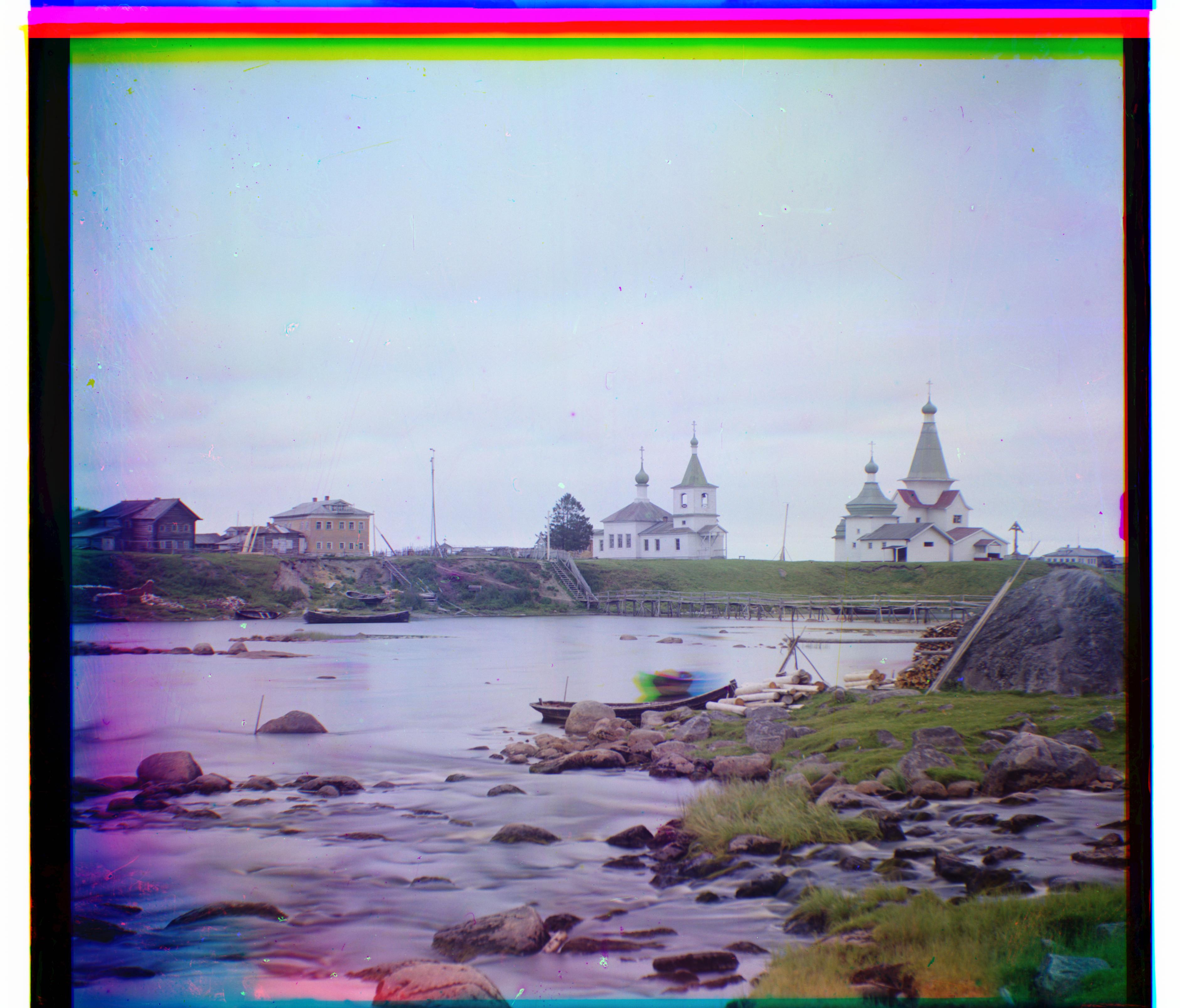
red offset = (121, -11), green offset = (35, -5)
Image link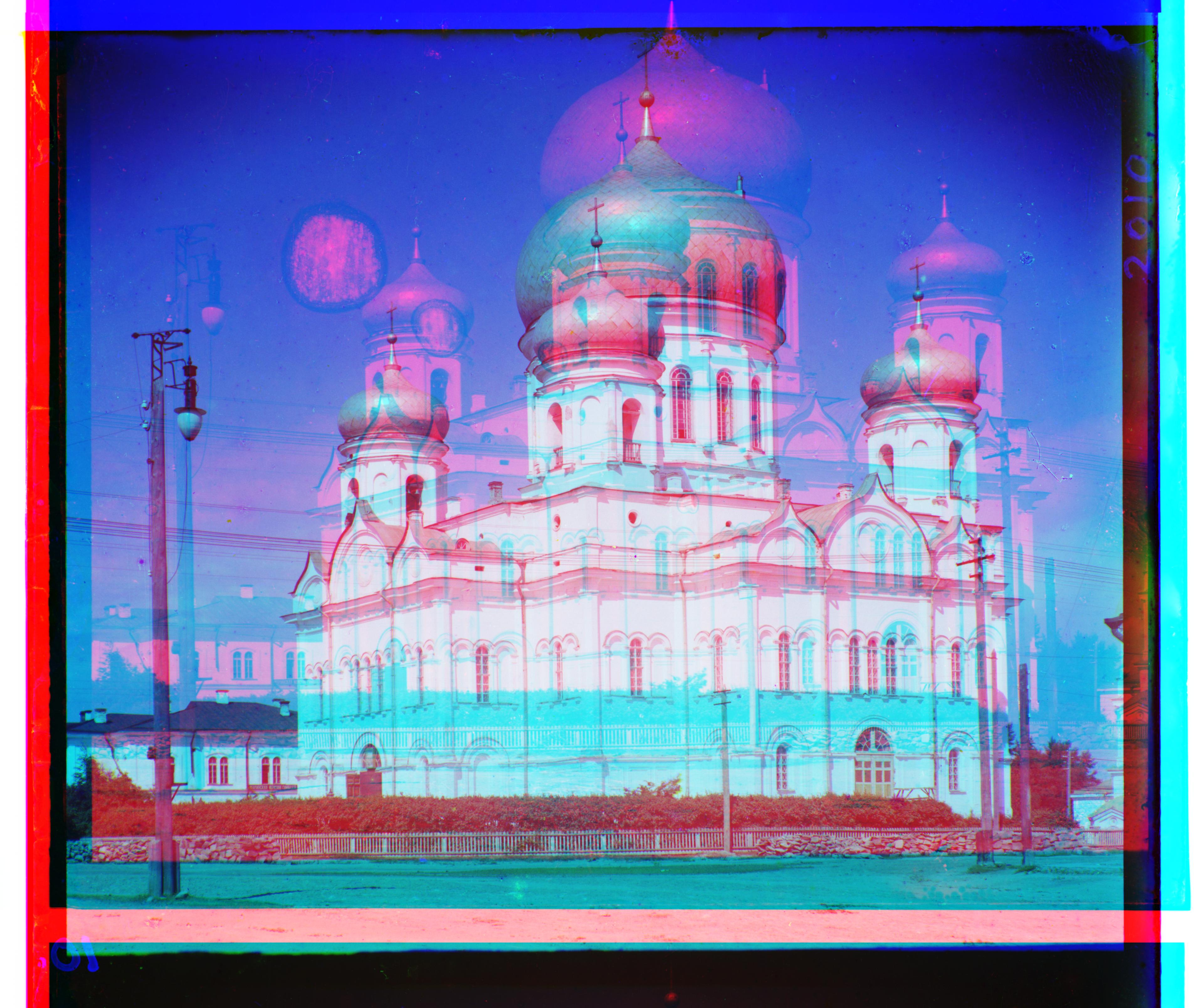
red offset = (-209, 67), green offset = (40, -7)
Image link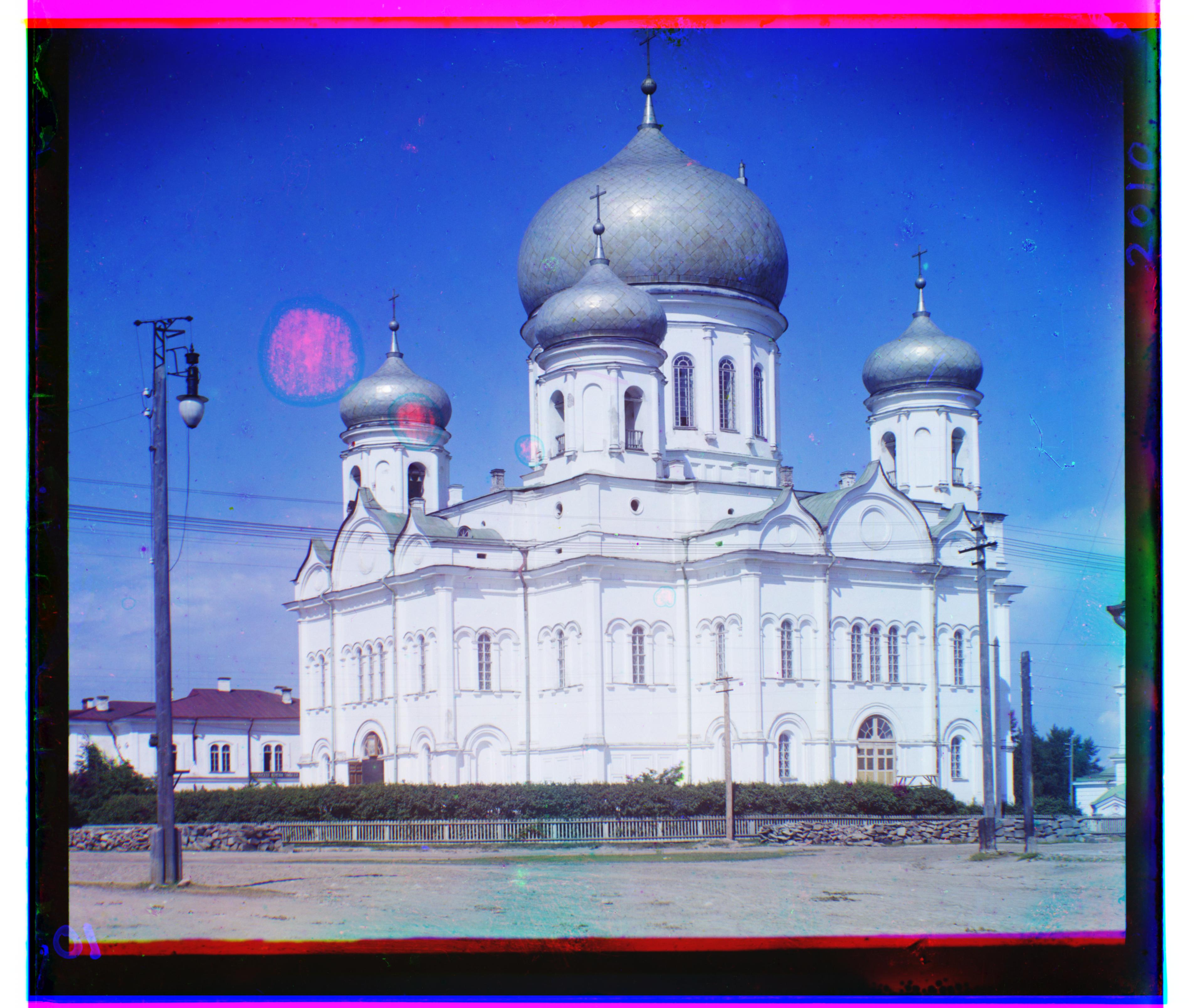
red offset = (90, -7), blue offset = (-40, 7)
Image link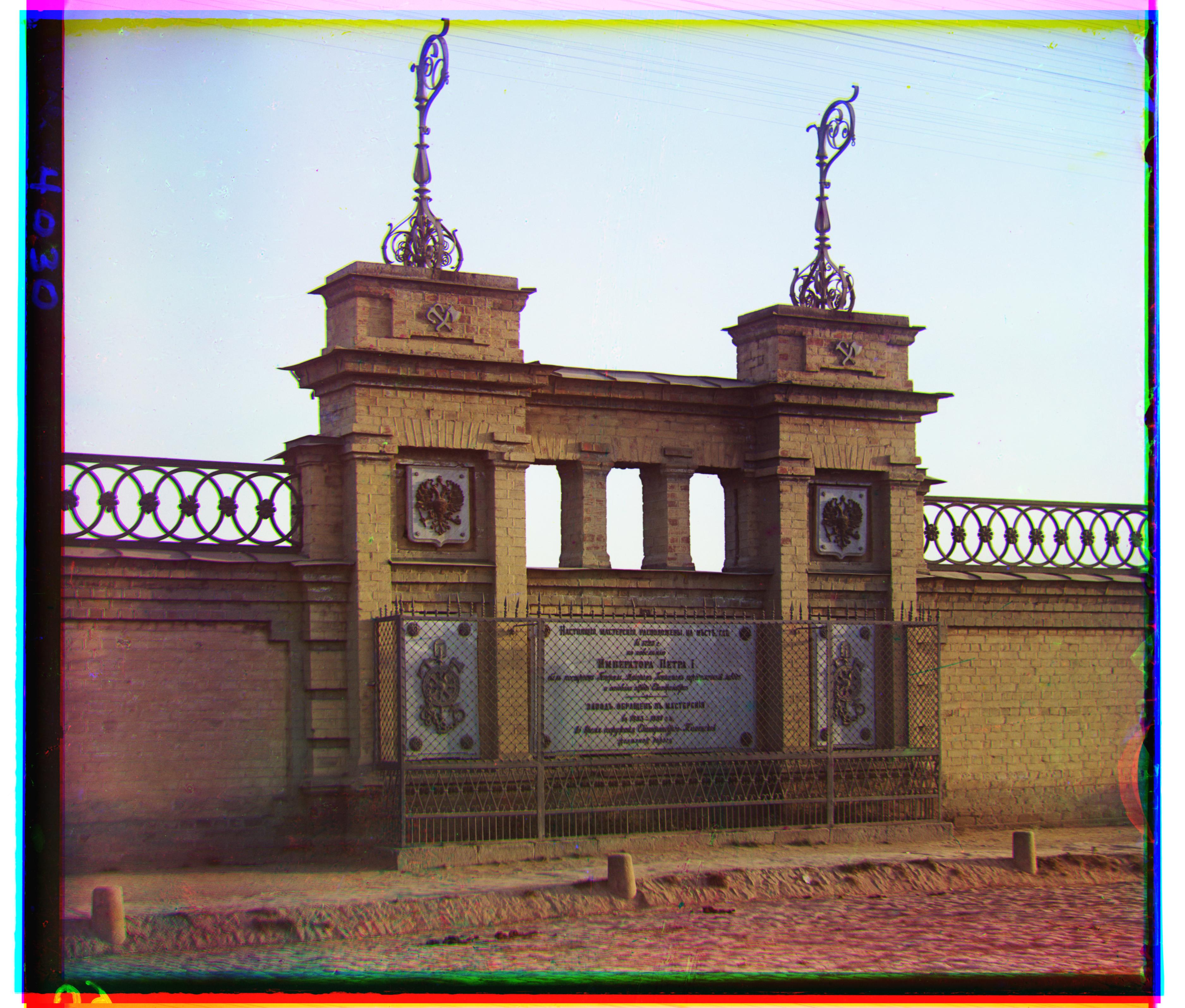
red offset = (105, -12), green offset = (53, -1)
Image link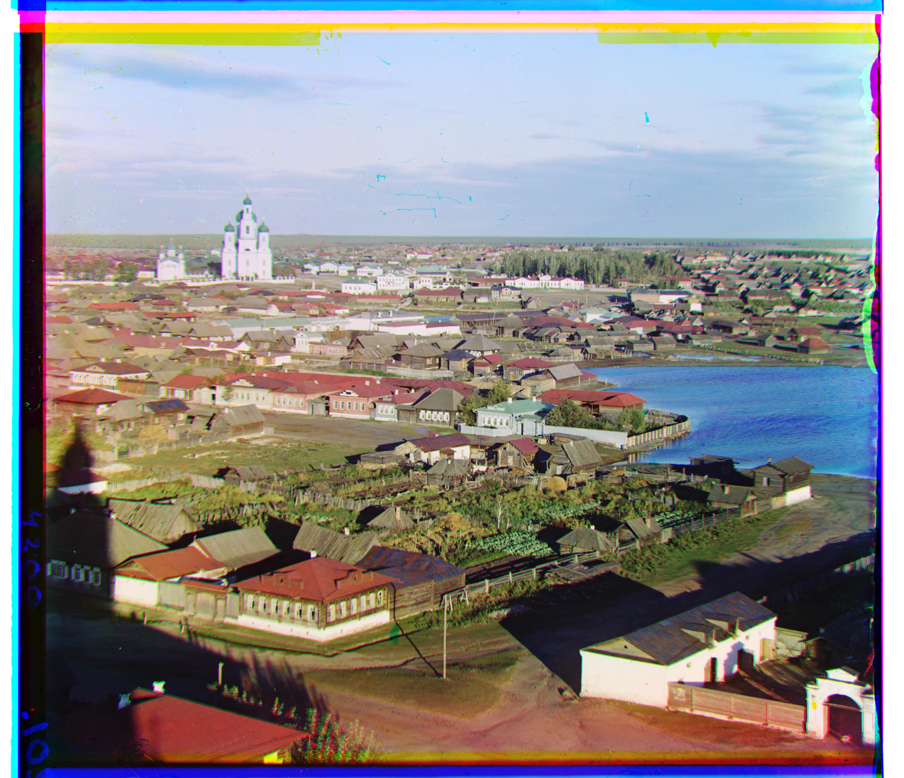
red offset = (134, -17), green offset = (59, -1)
Image linkFor auto cropping, I first trimmed my newly colorized image by its offsets before inputting the iamge into my autocropping function. For example, if an image had an offsets of (3, 4) and (-3, -2) I would input image[3:-3, 4:-2] into the autocropping function. I found this method to help extract weird stretchs of colors along the edges and helped the auto cropping function trim the white and black parts of the image better. Once this trimmed image is inputted into the function, the function looks at the first row and take the standard deviation of it for each image channel. If the average SD < 0.15, the first row is trimmed and we continue by looking at the second row. We continue this process until we reach a row with an average SD over the image channels > 0.15. After we trim the beginning rows, we retart this process but with the last row and working backwards, similarly trimming continuous rows with an average SD < 0.15. I then repeat this same process for the columns of an image. The following are results showing the effectiveness of the auto-cropping function.
For each of the two examples, I ran their individual image channels (r, g, b) through the cv2.canny function with the edge parameter = 100 and threshold1 parameter = 200. I then ran my multi-scale implementation with the outputs of the canny function acting as the images to align. Once I obtained offsets, I translated the original r, g, b images to obtain the new and better colorized image. Another cool thing to note is that I found the edge detection-centered multi-scale implementation to run ~7 times faster than the raw images.
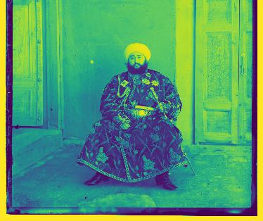
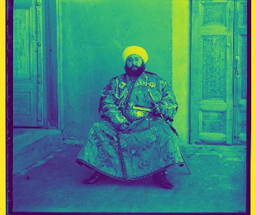
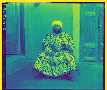
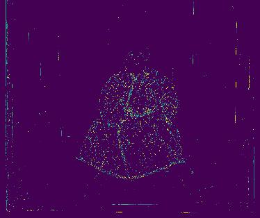
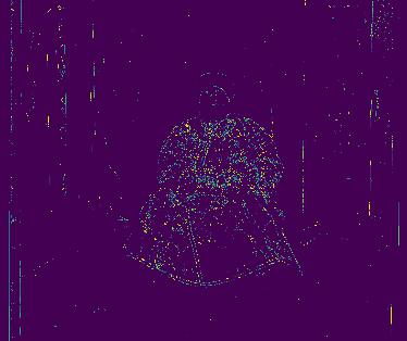
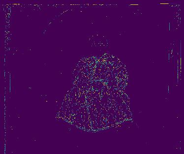
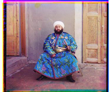
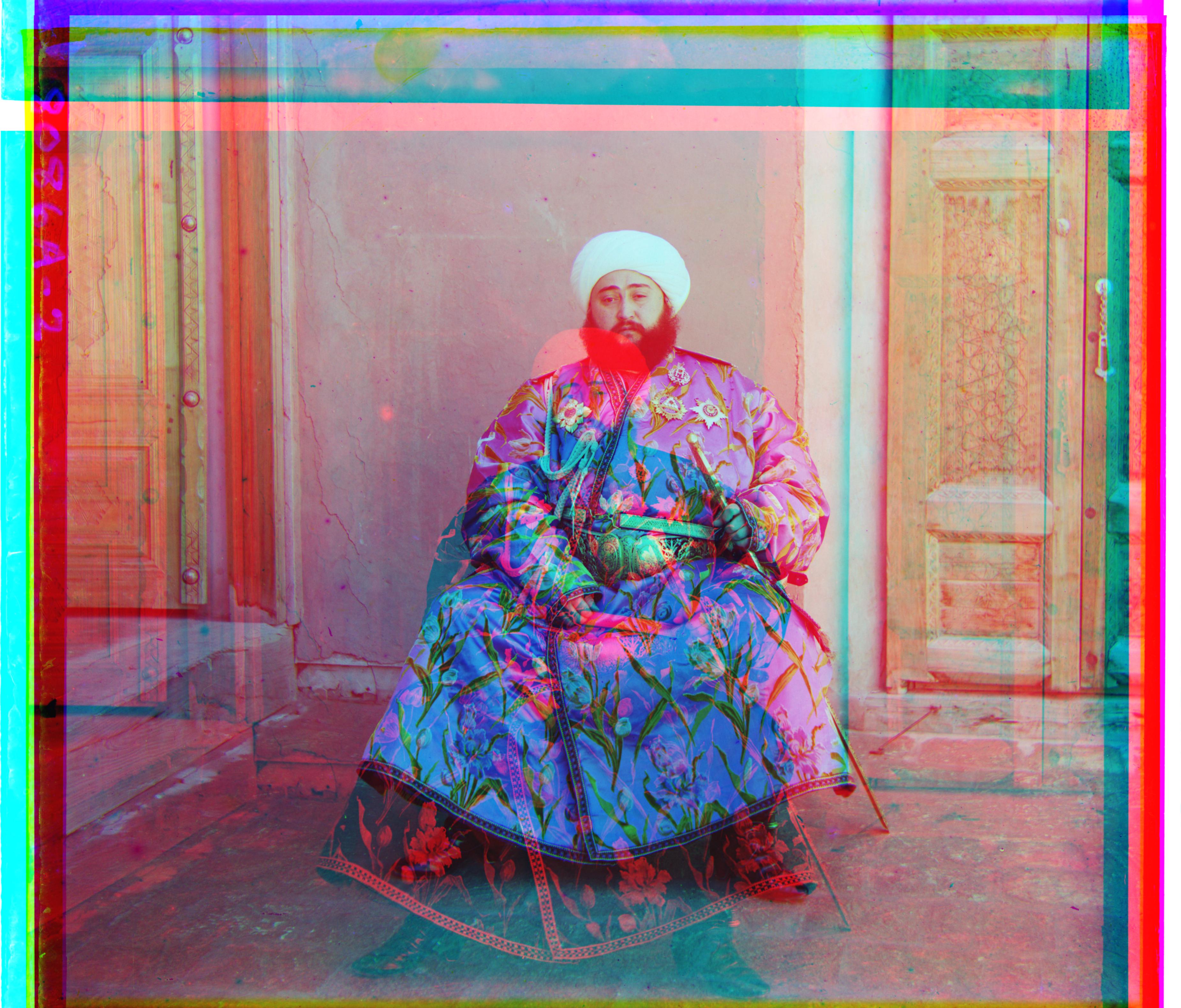
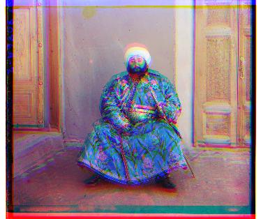
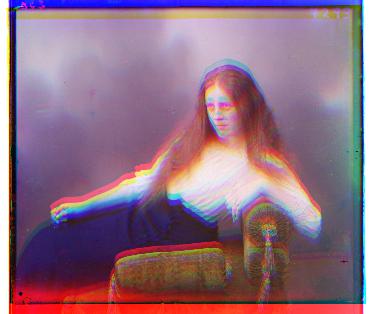
The multi-scale algorithm originally struggled with the emir.tiff image as the blue channel was found to not be the best as the base (the faulty resultant alignment is re-shown as the first image in the first row above.) This can be visually validated when displaying the r, g, and b image channels for the emir.tiff image (shown with images 2, 3, 4 respectively in the first row above). These images are visualized such that dark blue = the minimum of the image and yellow = the maximum of the image. We can see that using SSD to find the optimal alginment will cause problems with this image since the blue channel peaks in regions where the other filters don't necessarily peak (and vice versa). However, when displaying the edges of each image channel, we can see that these image channels are quite similar even if their pixel intensities differ greatly. The edge detection outputs for the r, g, and b image channels are shown in the first 3 images in the second row above. When using these edge detection outputs as the inputs for the multi-scale implementation, the blue channel was able to successfully act as the base. The edge detection alignment is displayed as the last picture in the second row above. The offsets for it were red offsets = (107, 41) and green offset = (49, 24).
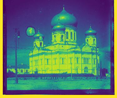
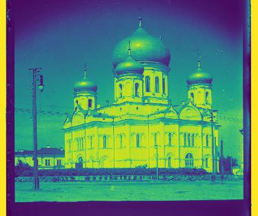
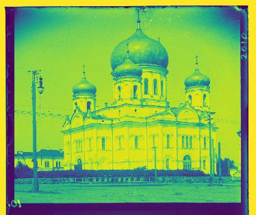
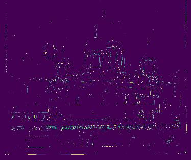
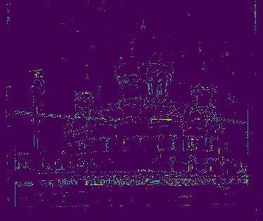
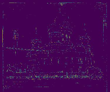
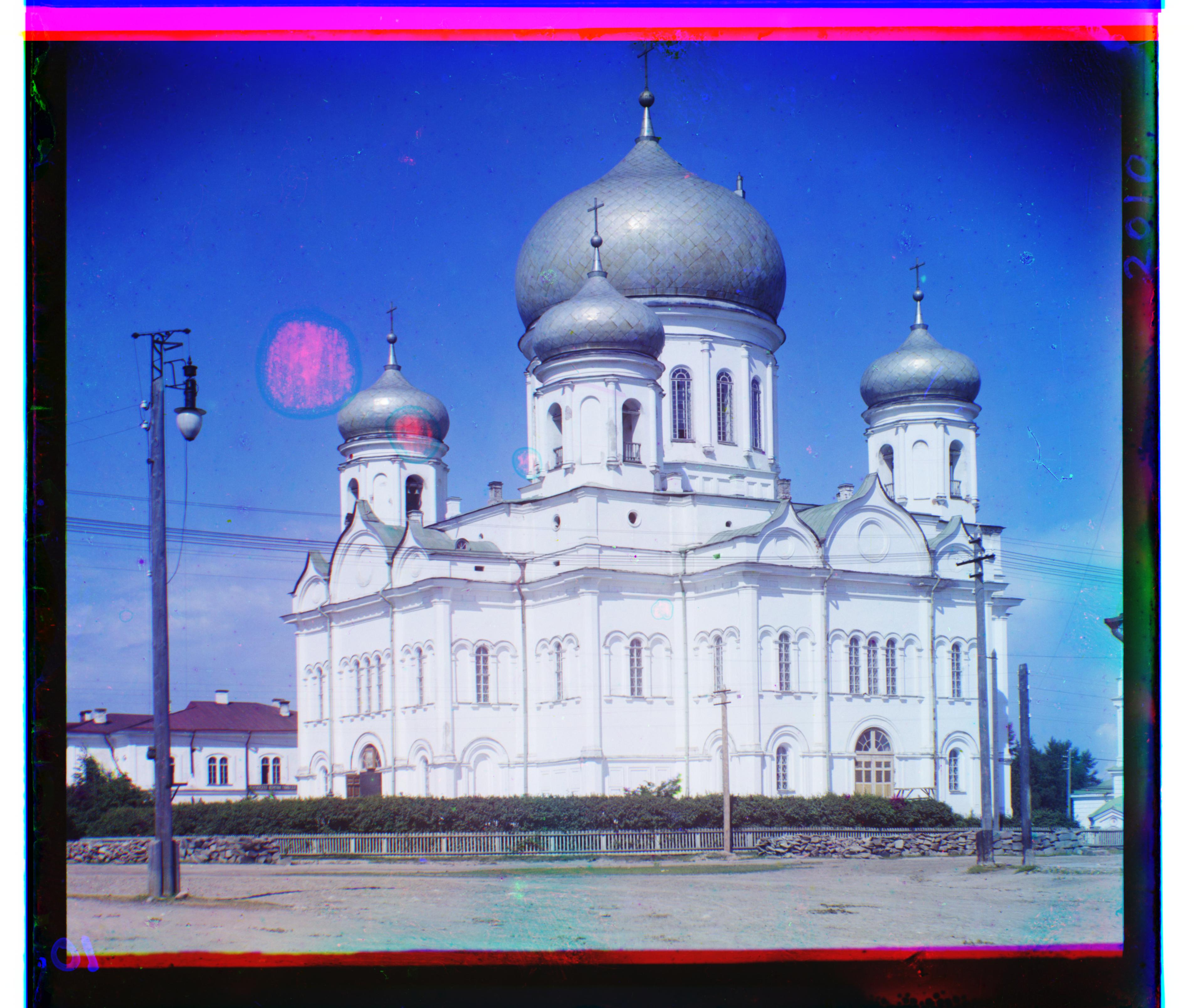
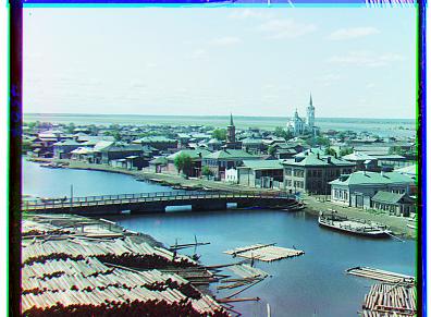
The multi-scale algorithm similarly struggled with the petrozavodsk church.tiff image as the red channel had some damages and once again the blue channel differed right now on an intensity basis from the two other image channels. This can be visually validated when displaying the r, g, and b image channels for the petrozavodsk church.tiff image (shown with images 2, 3, 4 respectively in the first row above). These images are visualized such that dark blue = the minimum of the image and yellow = the maximum of the image. Once again, when displaying the edges of each image channel, we can see that these image channels are quite similar even if their pixel intensities differ greatly. Even though the red image channel had some damage to it, the edge detection filter was able to help the multi-scale implementation align the image channels better than it had dome before. The edge detection outputs for the r, g, and b image channels are shown in the first 3 images in the second row above. The edge detection alignment is displayed as the last picture in the second row above. The offsets for it were red offsets = (130, -15) and green offset = [40, -7].
For this section I was interested in seeing how better alignment between image channels would impact OpenAI's CLIP's output. Specifically, I restricted the dataset given to us to a smaller set (lady.tiff, emir.tiff, monastery.jpeg, onion_church.tiff, tobolsk.jpeg, three_generations.tiff, workshop.tiff) and converted their image file names into "labels" (so that smaller set of images created the following label list -> ["an emir", "a lady", "a monastery", "a onion church", "three generations", "the city tobolsk", "a workshop"]). Then, the naive concatentation and project-output alignment were both run through CLIP to see the text label distribution for both images and see if there were any difference. From this small experiment it can be seen that better alignment always improved the probability for the correct label. Results for the specific images are below in their respective sections. It would be cool to expand this project to include more images to see if this is true overall. The code used to obtain the CLIP output distributions were taken from the CLIP Github page.
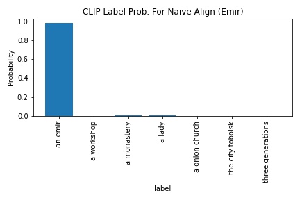
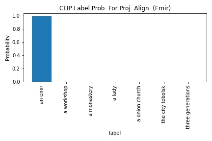
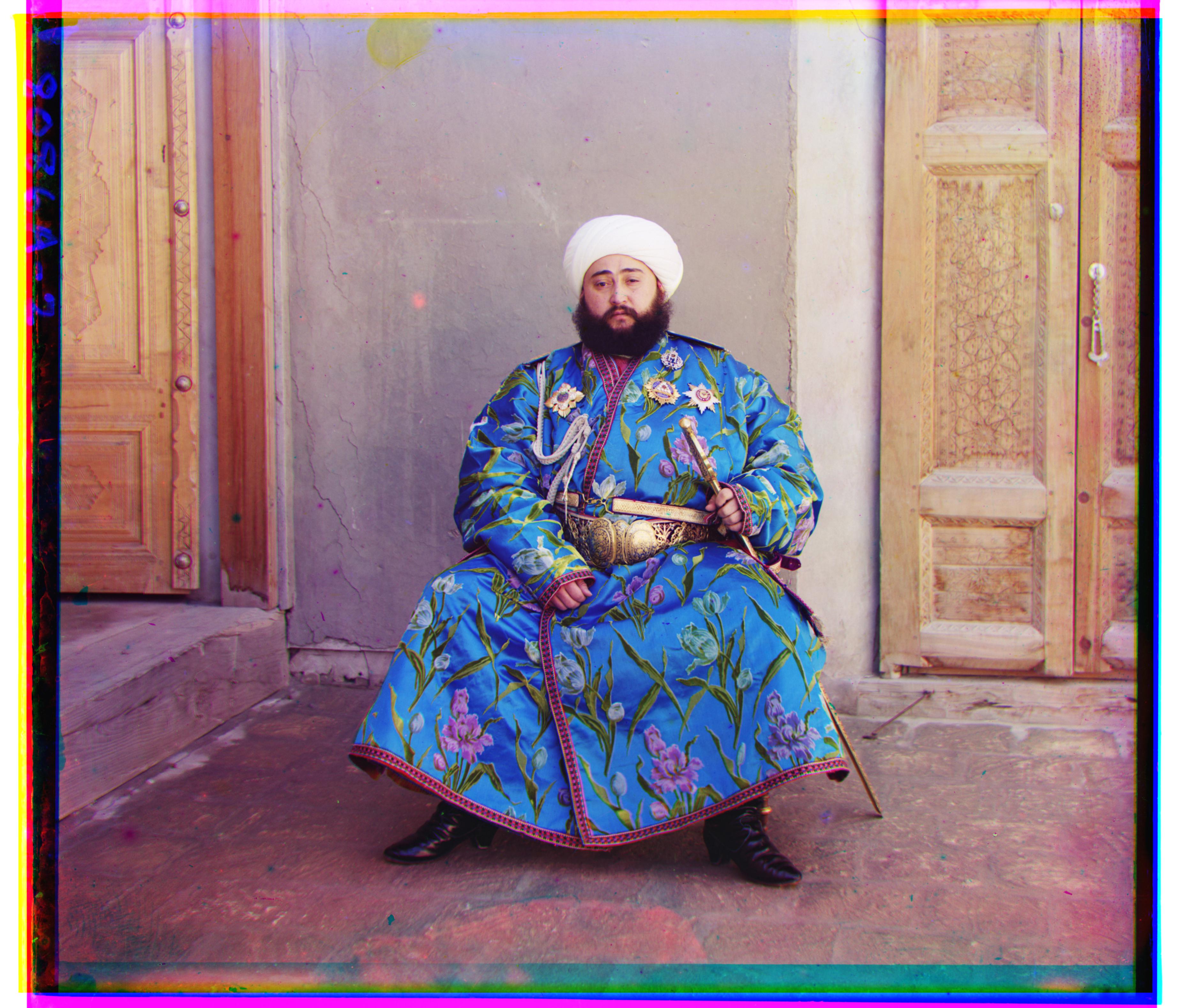
CLIP's probability in outputting "a emir" increased from 97.9 to 99. The edge detection-blue base output was used as the project-output alignment for this section.
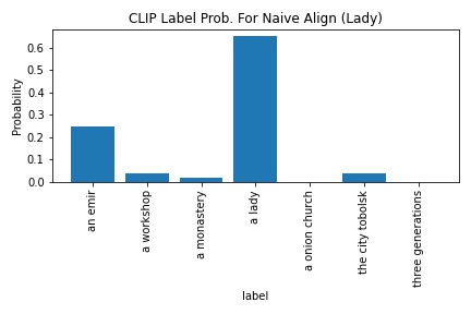
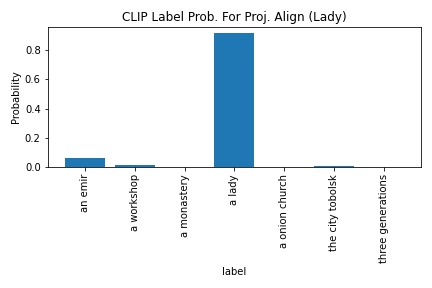
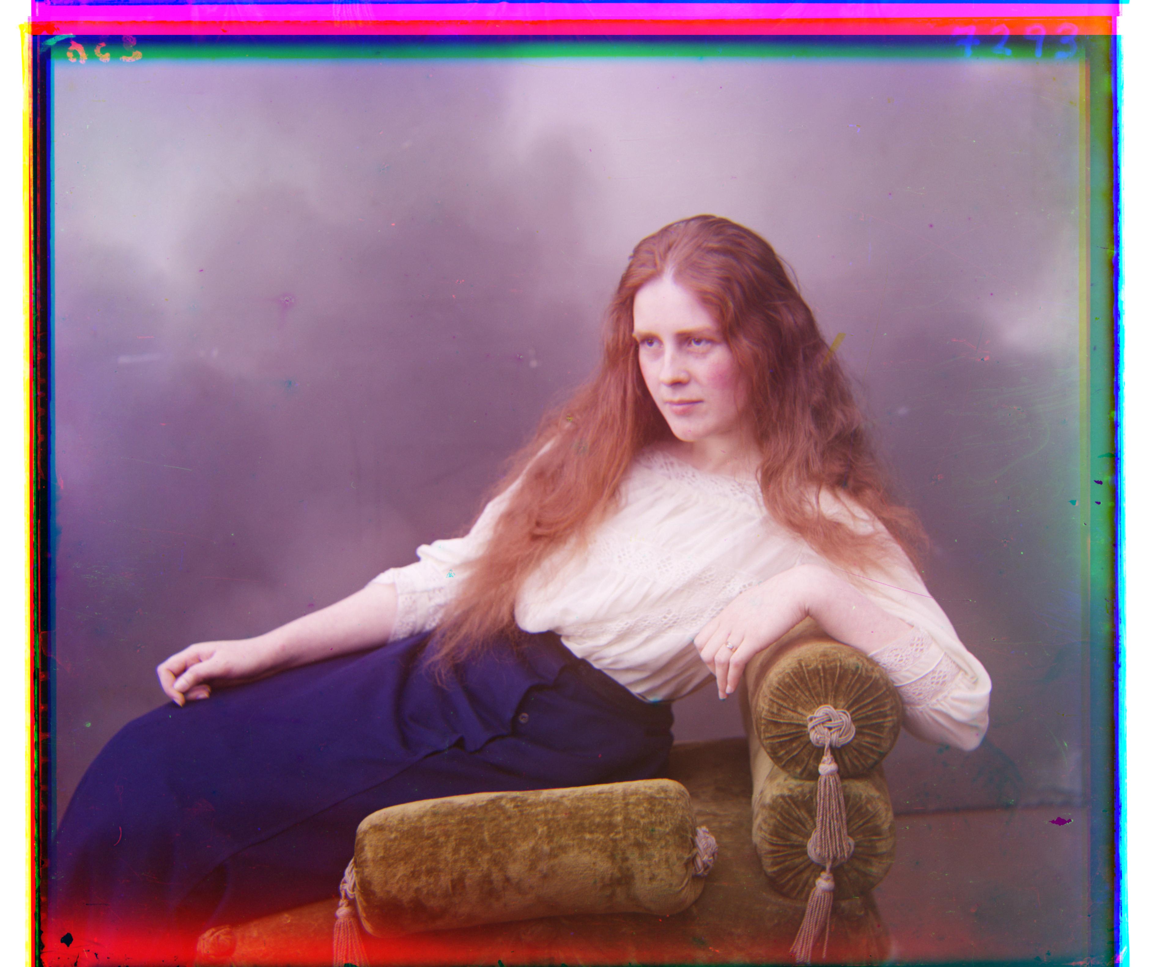
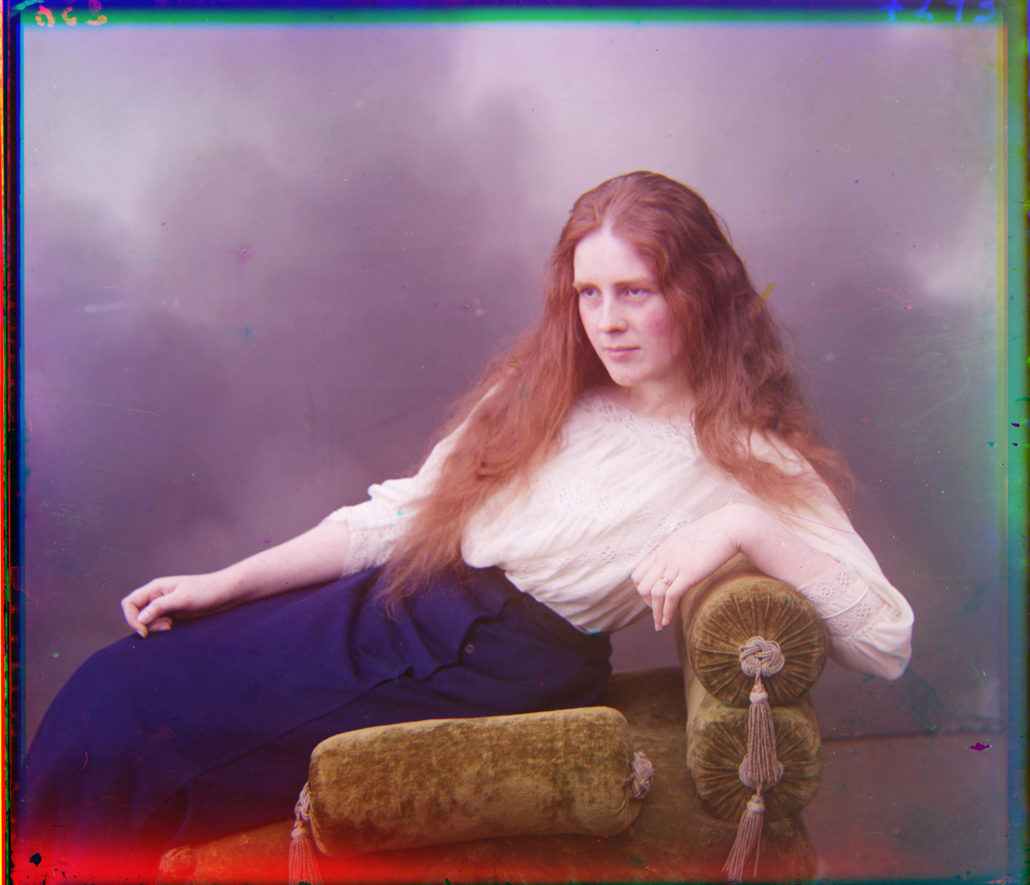
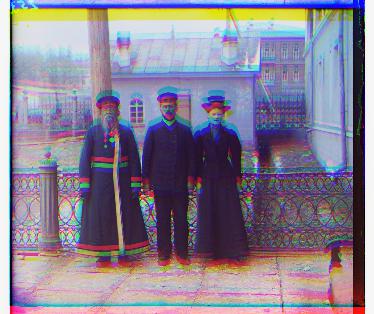
CLIP's probability in outputting "a lady" increased from 65.1 to 91.4. It was really interesting how the probability increased enough to cause the lady.tiff image to be a strongly given the "a lady" label. Moreover, I wonder if adversarial examples could be effectively created from just translating/offsetting image channels.
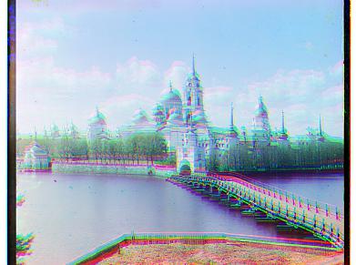
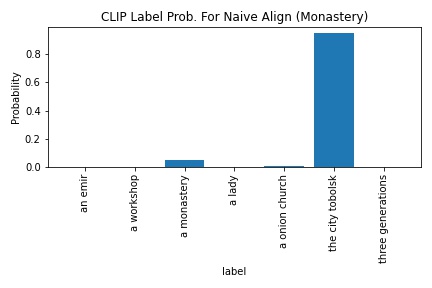
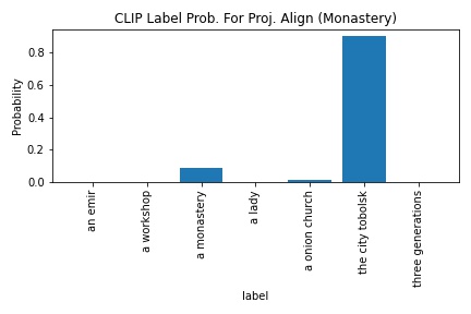
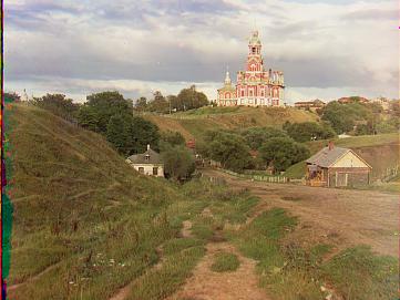
CLIP's probability in outputting "a monastery" increased from 4.7 to 8.6. Since the image resolution was smaller and there were other possible labels, I wasn't too surprised by the low probability. However, the better alignment still was able to drag the "a monastery"'s probability slightly higher.
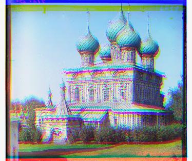
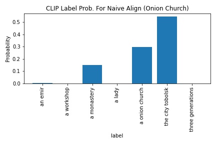
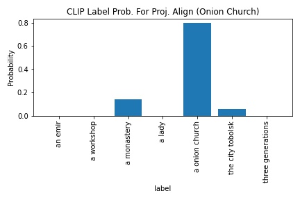
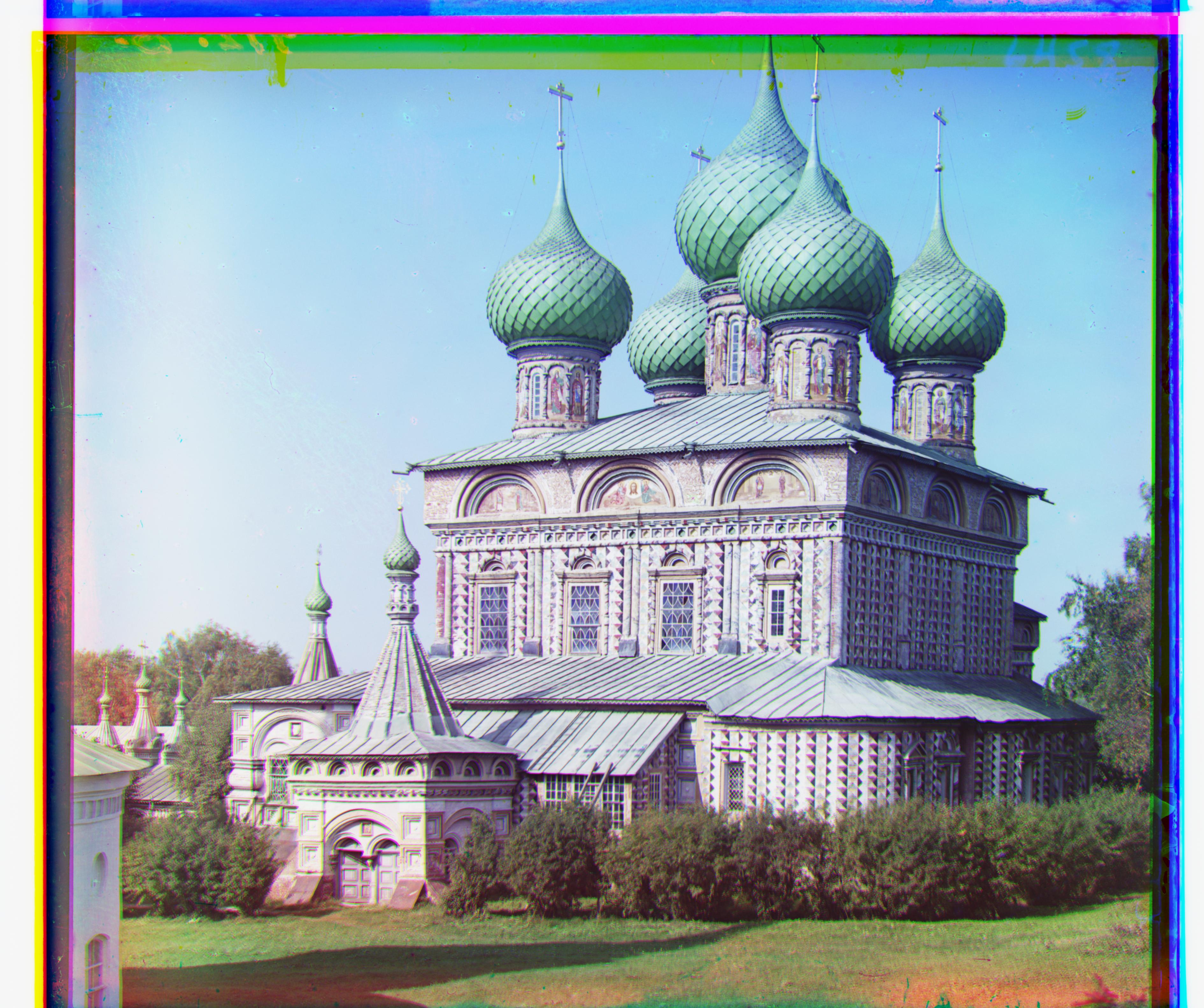
CLIP's probability in outputting "a onion church" increased from 30.0 to 79.5. I was really surprised how the naive image could have been considered an adversarial example when the better aligned image had much better results.
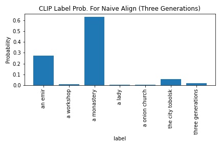
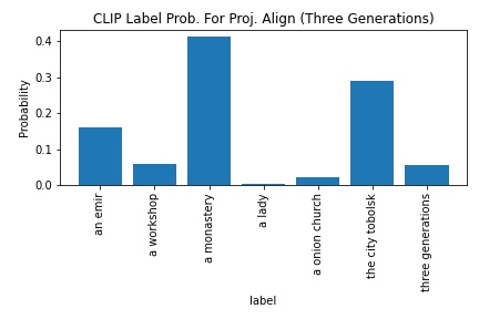
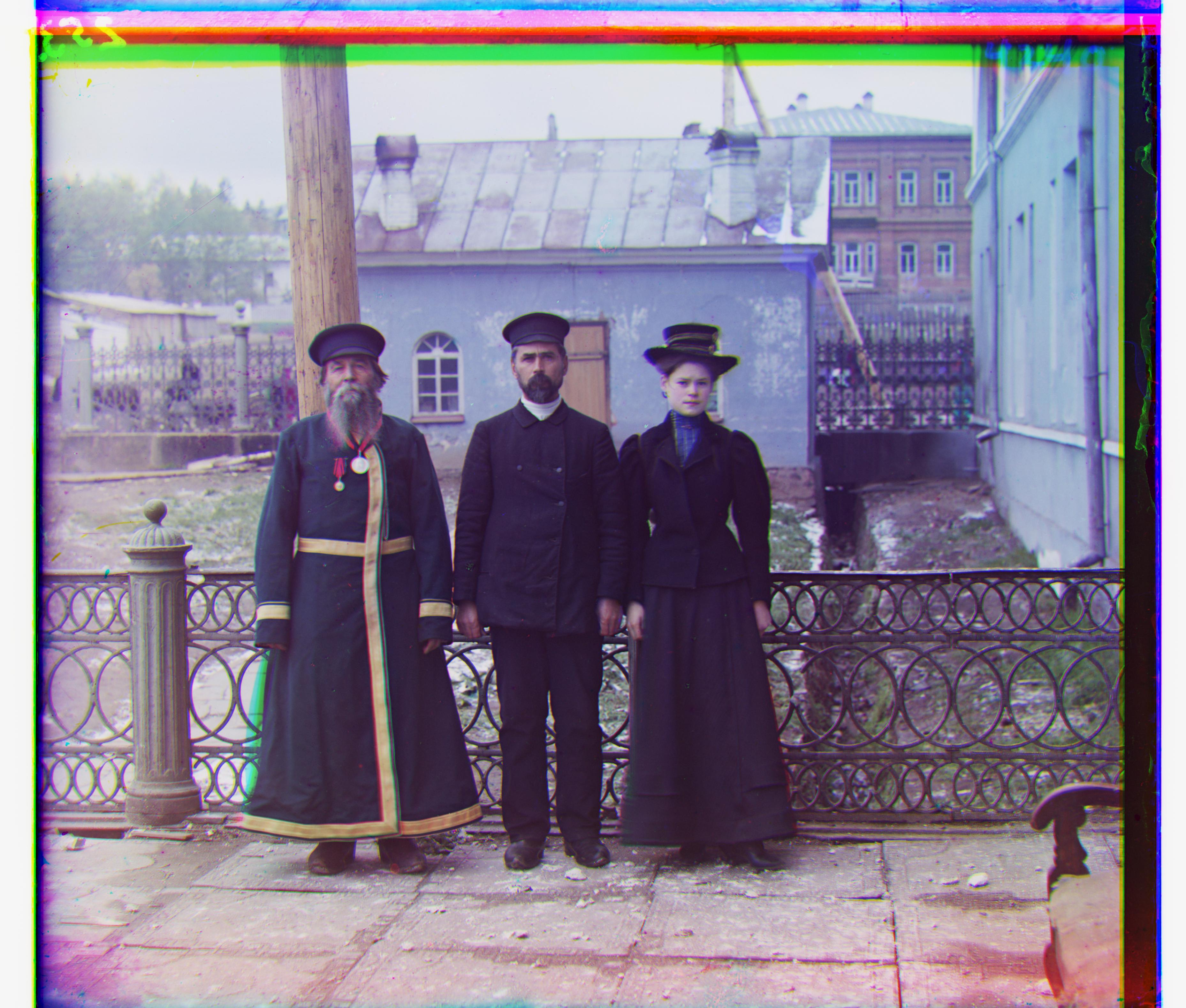
CLIP's probability in outputting "three generations" increased from 1.7 to 5.5. Similarly to the monastery.jpeg's outputs, I wasn't too surprised by the low probability. Still really cool how better alignment by itself was able to drag the "three generations"'s probability slightly higher.
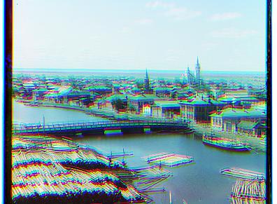
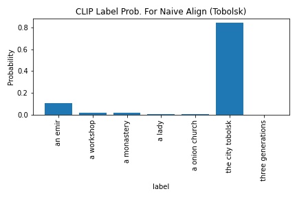
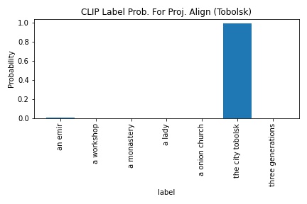
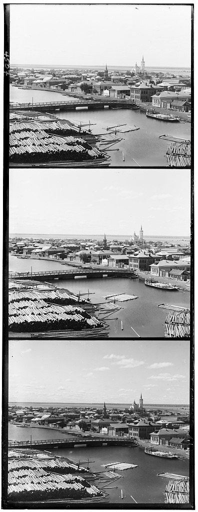
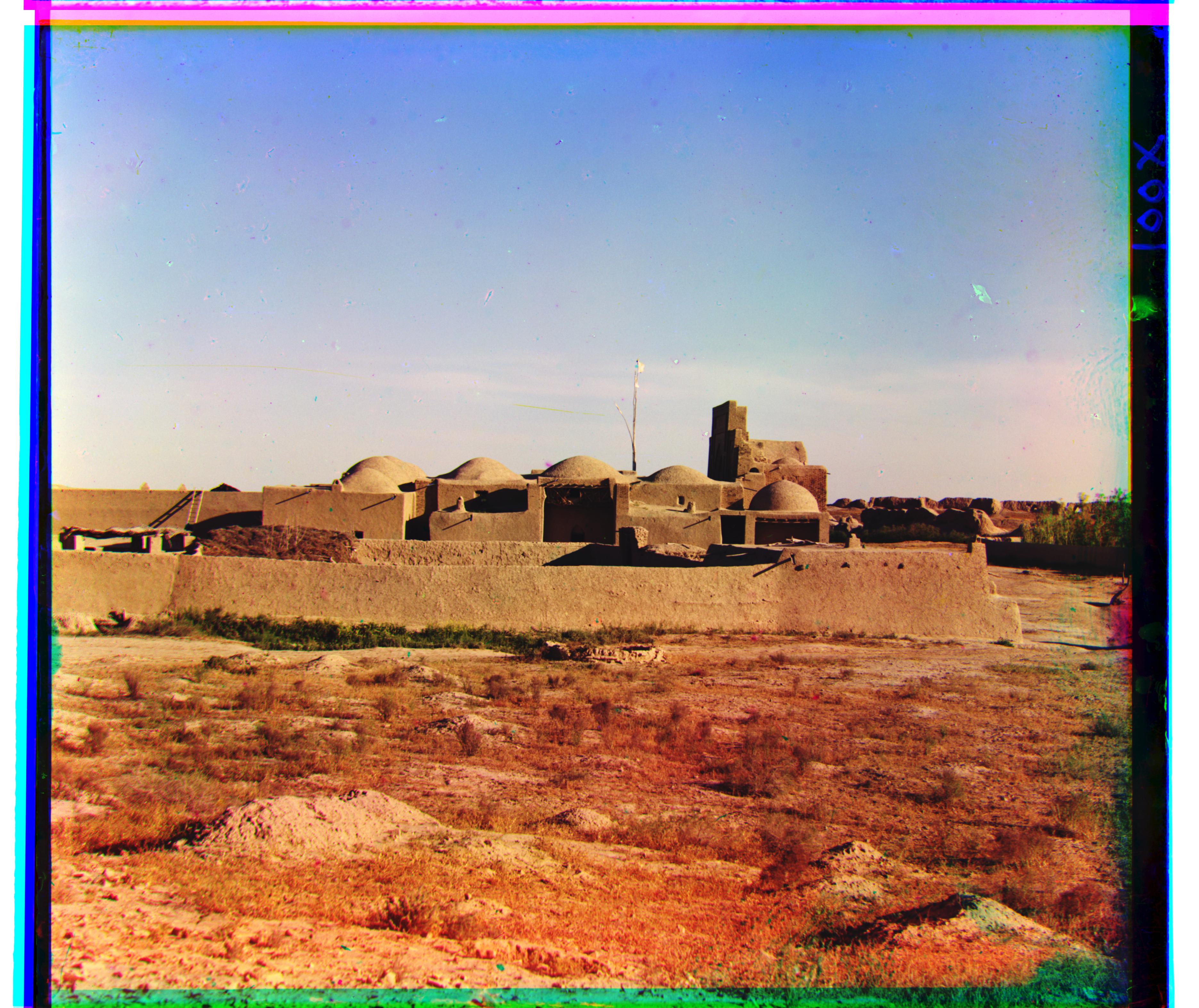
CLIP's probability in outputting "the city tobolsk" increased from 83.9 to 98.7. Even though "the city tobolsk" is the most logical label for the image given the set of image labels, it was interesting how confident CLIP was even with the image mis-aligned.
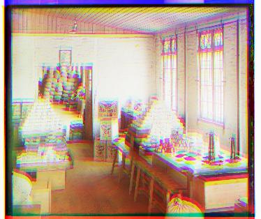
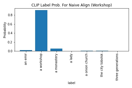
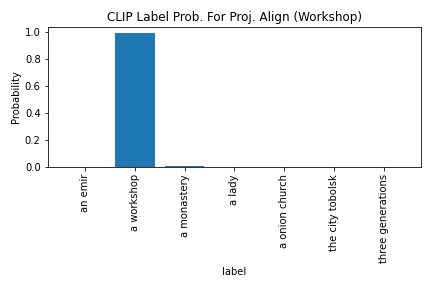
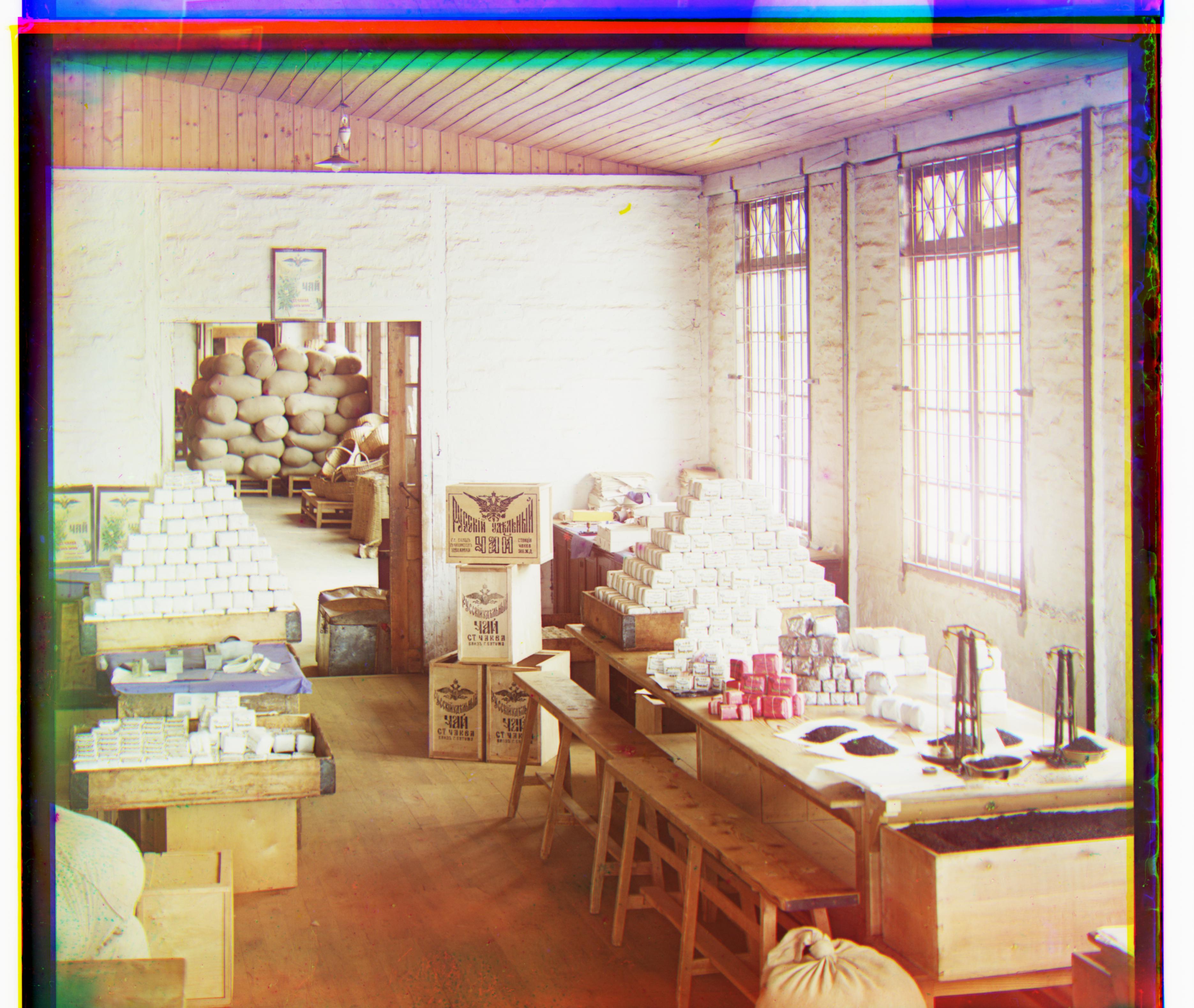
CLIP's probability in outputting "a workshop" increased from 90.5 to 98.8. The edge detection-blue base output was used as the project-output alignment for this section.