In the early 20th century, prior to the Bolshevik Revolution that overthrew the Tzar empire of Russia and established the Soviet Union, a pioneering photography named Sergei Mikhailovich Prokudin-Gorskii sought to take color images of the Russian countryside to be used in education institutions. His approach was to take three separate images of the same scene but on each shot applying a different color filter; a red, green, and blue filter were used. The task of this project was to use the negatives of these three color channels, align the three color channels together and then stack them in order to reproduce the final color image as it was intended to be seen in schools across the Russian Empire.
The three image alignment metrics which I implemented were sum of squared differences, normalized cross-correlation and zero normalized cross-correlation. All three metrics yielded extremely similar results; thus, in favor of the significantly reduced computational overhead associated with the sum of squared differences metric, it was my metric of choice to produce the final images. For the smaller negatives, exhaustive search was sufficient to find the proper alignment of the three color channels; however, for the much larger tif image negatives, exhaustive search proved to be too slow to find the proper alignment which ranged sometimes over 100 pixels. The solution to processing the higher resolution negatives was to implement a pyramid search which afforded the narrowing of the bounds used for naïve search at each scaled layer of the original negative, compounding and scaling the corrections as the pyramid search moved from the top of the pyramid (the layer which scaled down the negatives the most) to the bottom of the pyramid (the layer which held the original resolution of the negatives).
I will proceed to briefly explain the implementation details of each metric used for computing the image alignment scores for the color channels in addition to the performance improvement afforded by the pyramid search algorithm.
There were three image alignment metrics which I implemented. The first is sum of squared differences (SSD) which begins by applying an element-wise subtraction function between the two images. The algorithm first subtracts every value from the first image with every value from the second image. This is an element-wise subtraction so that each value stored in an (x,y) position in the first image is only subtracted by the corresponding value stored in the same (x,y) position of the second image. One the difference matrix is computed, each value in the matrix is squared, getting rid of negative values, and then every value in the matrix is summed to produce a final output value. If the two images are identical, then the resulting difference for each pixel would be 0, e.g. the value stored at each (x, y) position in the matrix would be 0 and so the resulting sum squared difference score would be 0. A higher sum of squared differences score, the less similar the two images are; thus, our search algorithm when using the sum of squared differences metric is to minimize the returned value for the best alignment.
The second metric used is normalized cross-correlation (NCC) which is computationally the dot product of the two images whose vectors have been normalized. I implemented this method by solving for a quotient with the value of the numerator computed by multiplying the two images together (element-wise) and then summing their values and the denominator computed by squaring and summing across every value in each image, multiplying the two summed image values and then taking the square root of the product. I confirmed that both approaches returned the same metric scores but since high-level operations were not allowed in this project, the latter approach was used for actual computations. Unlike the SSD metric, the NCC metric favors a higher score with a value of 1 signifying a perfect image match.
The third metric used is zero normalized cross-correlation (ZNCC) which is very similar to NCC except that the average of each image is first subtracted from each respective image matrix prior to performing the aforementioned operations. The same principle holds for ZNCC as for NCC that a value of 1 signifies a perfect image match, which is the highest value that can be returned from either NCC and ZNCC.
The images displayed later on were generated using the SSD metric which I determined to be my metric of choice simply because NCC and ZNCC did not offer a significant improvement over SSD in terms of image quality; in fact, while testing the smaller negative image files the correction vectors were identical across all three metrics. Meanwhile, SSD was computationally less expensive which was an important factor when implementing pyramid search resulting in approximately a 20 second speed-up when compared to using NCC and ZNCC.
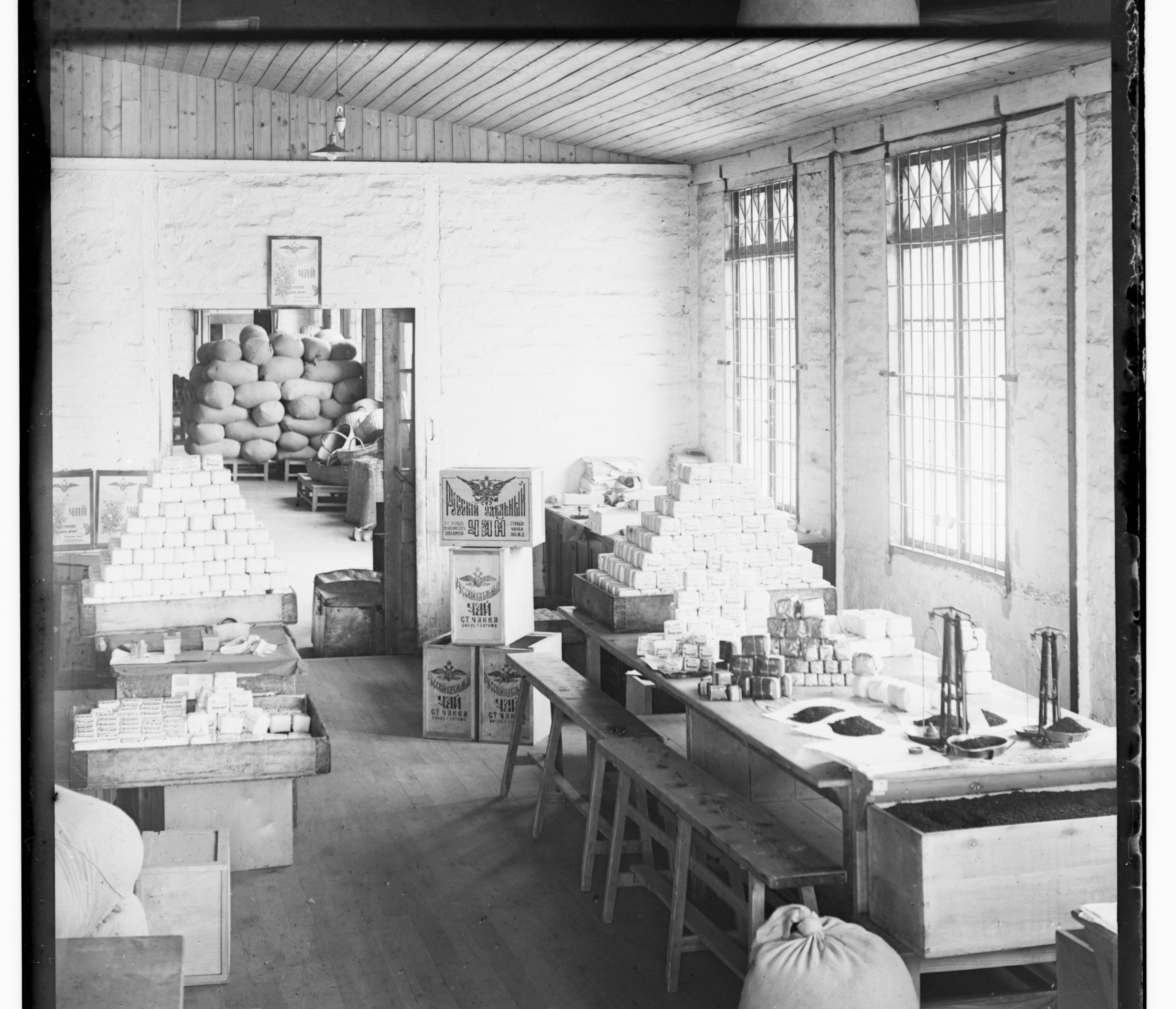
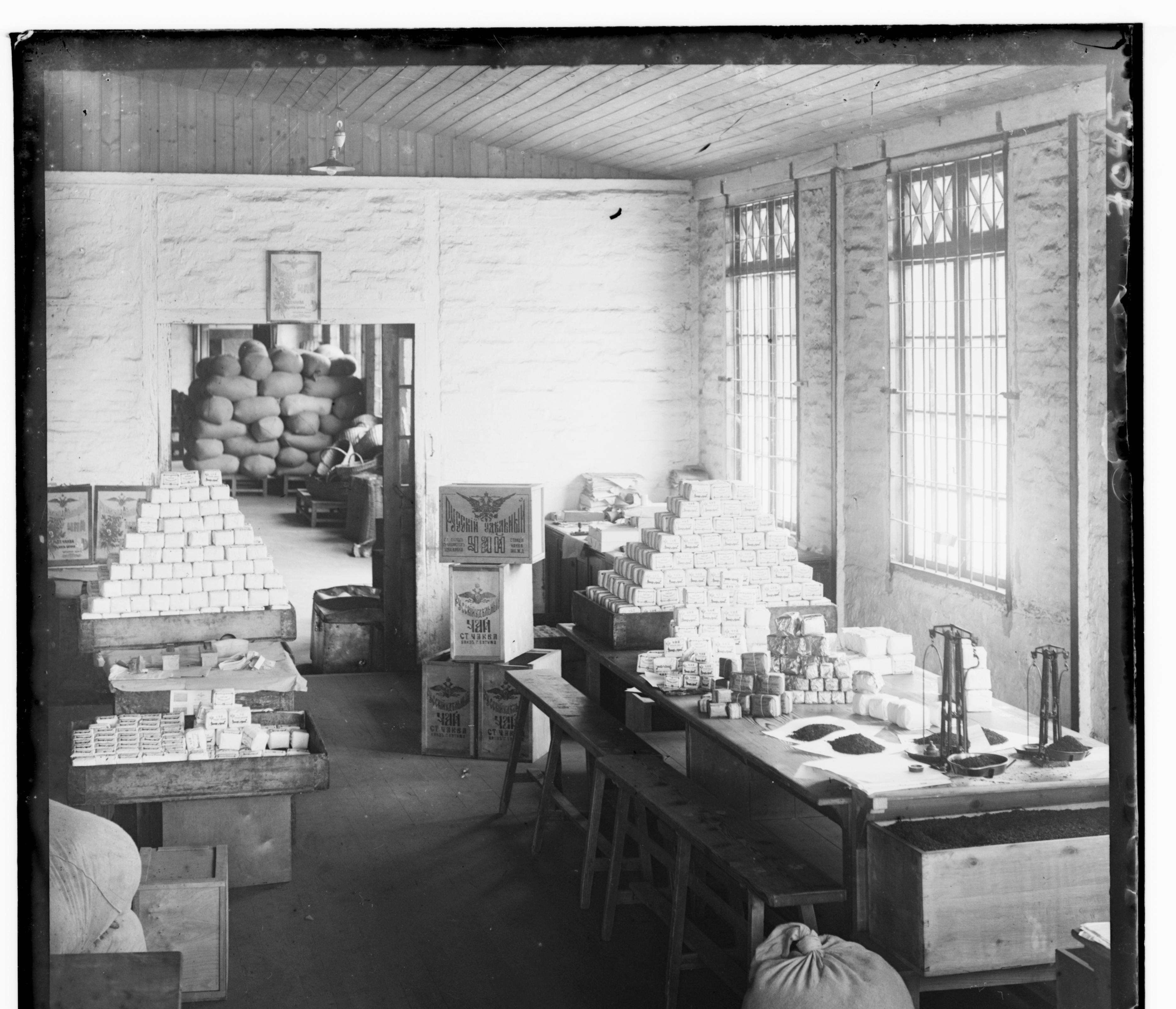
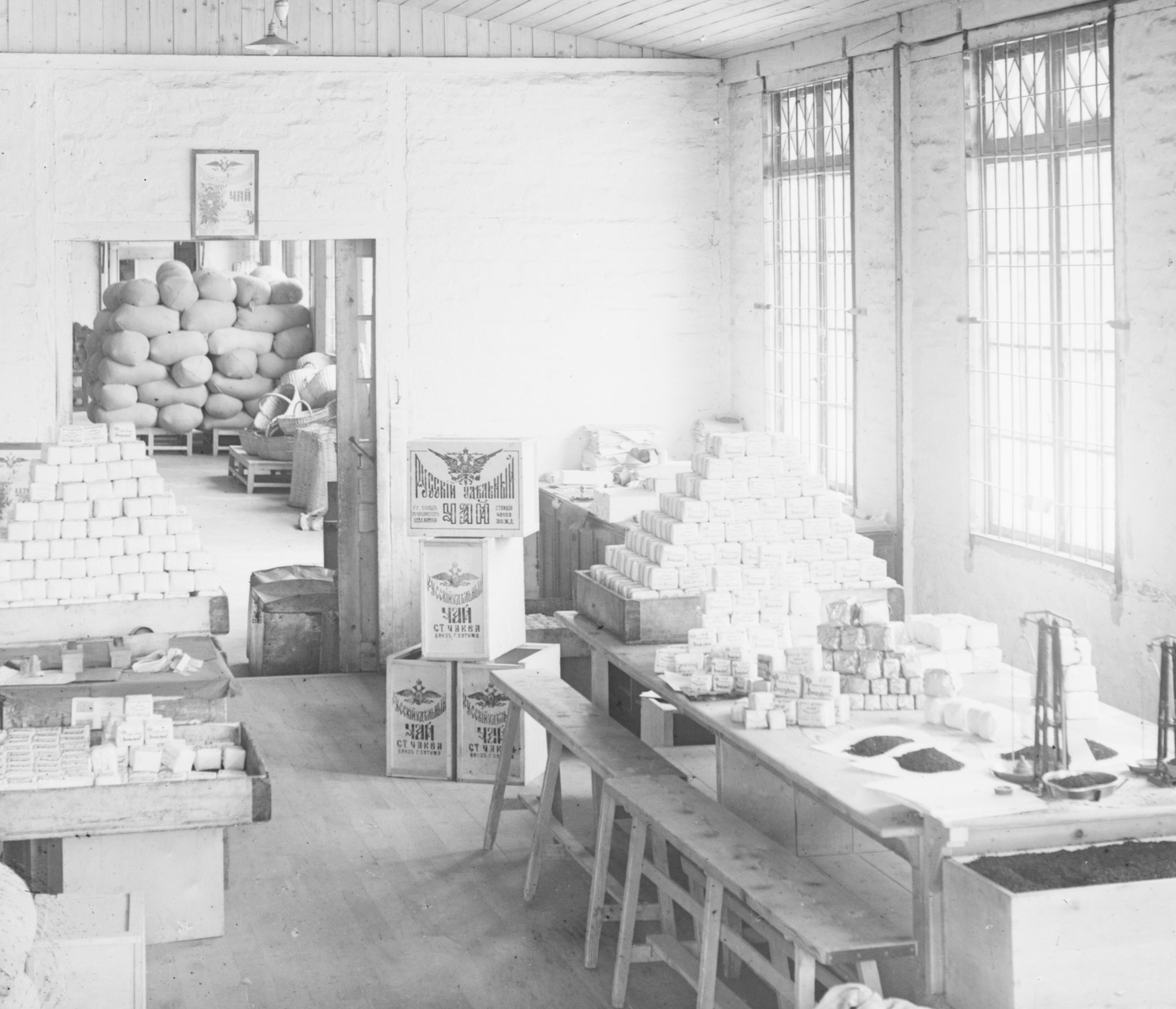
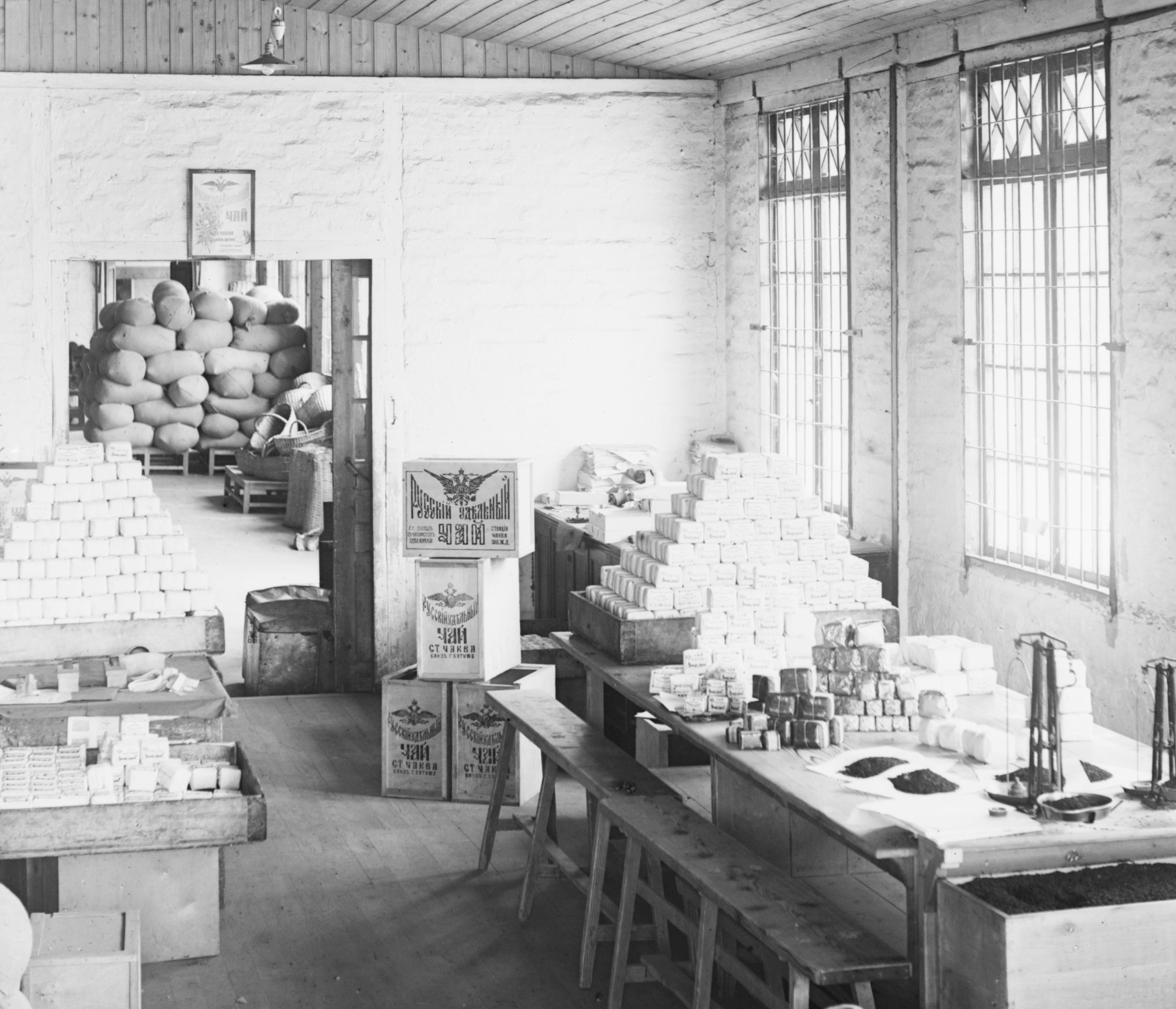
A common challenge I faced early-on was that the correction vectors produced from all three metrics resulted in color images that were not even remotely stacked appropriately. To resolve this issue, after spending several hours scrutinizing the implementation of each metric, I determined that the noise around the perimeter of each negative was significantly influencing the alignment metrics, resulting in an incorrect selection for the correction vector. Prior to running either exhaustive search or pyramid search on the negatives, I crop the perimeter noise around the negatives and apply the matching algorithms on the cropped images to obtain the correction vectors, which are then applied to the original, uncropped negatives. I decided to crop 10% off of each side of the image so that the alignment algorithm could focus on the contents of the image rather than the perimeter noise. Below are example images of each color channel showing how the color channels looked prior to cropping and how they looked after cropping.

The naïve approach to aligning the three color channels from the provided negatives was to perform an exhaustive search shifting all the pixels in one of the images by a certain amount defined by the range [-15, 15]. This was done using the numpy function np.roll and translations were applied separately to both the x and y axis of the image, using nested loops (one for the x translation and one for the y translation) accounting for all possible combinations of x and y pixel shifts.
Exhaustive search worked well and was very quick for the low-resolution negatives. The three colored images from low resolution negatives created using exhaustive search are displayed below. The images were produced using the green color channel as the base channel to which the red and blue color channels were matched. Though on the lower resolution negatives the choice of base channel used has insignificant effects on the final output of the color image, there was a much more noticeable effect on final image quality from the high resolution negatives which I will explain shortly.
When it came to higher resolution negatives, exhaustive search proved to be prohibitively expensive since the range of potential shifts in both the x and y directions would have to span at least [-150, 150]. To overcome this issue, we implemented a pyramid search algorithm which progressively scaled down the high-resolution negatives at each level of the pyramid and then, starting from the top level (most scaled down version of the negatives) the exhaustive search was applied on a tighter range of potential shifts. Moving up each level of the pyramid also meant the correction vector from the previous level had to also be scaled by the same amount the negatives were downscaled. This search method enables for a correction vector to be found much more quickly than applying exhaustive search to the only the original resolution negatives and my implementation averaged around 40 seconds to execute.
After some experimentation, the pyramid search parameters I settled on were an exhaustive search ranging [-5, 5] at each level of the pyramid and the pyramid would contain 4 levels and at each level going up the pyramid, the image was scaled by 0.5. Again, for the alignment metric I utilized SSD instead of NCC or ZNCC because SSD provided an equally good color image quality and also had significantly less computational overhead, speeding up the execution of pyramid search. An issue I did notice on some of the images was that pyramid search did not quite find the best alignment for the green and red color channels which was an issue I resolved by experimenting with changing the base color channel. I explain more about my observations in the following section. Images generated using pyramid search can be found in the section titled Image Gallery. Additionally, all of the correction vector outputs from exhaustive search and pyramid search can be found in the Correction Vectors Table section.
In the project specifications, we were instructed to use the blue color channel as the base color and match the red and green color channels to the blue one. However, even though this technique worked well for the low-resolution negatives, some of the higher resolution negatives did not align perfectly, resulting in some color haze around boundaries. Initially thinking there was something wrong with my implementation of the pyramid algorithm, I tried numerous different parameters, changing the number of levels, the range of pixel shifts for each level used by the exhaustive search, and the scaling value, some of which made improvements to the generated images at the expense of runtime, sometimes exceeding 5 minutes of computation.
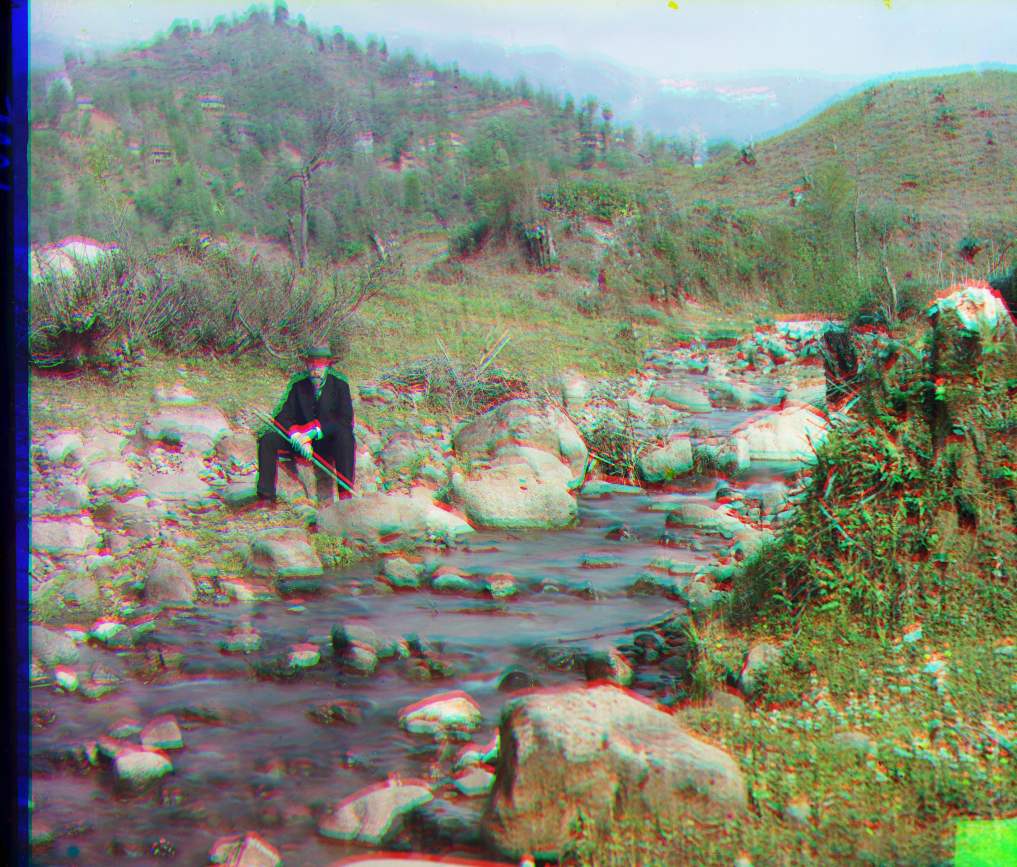
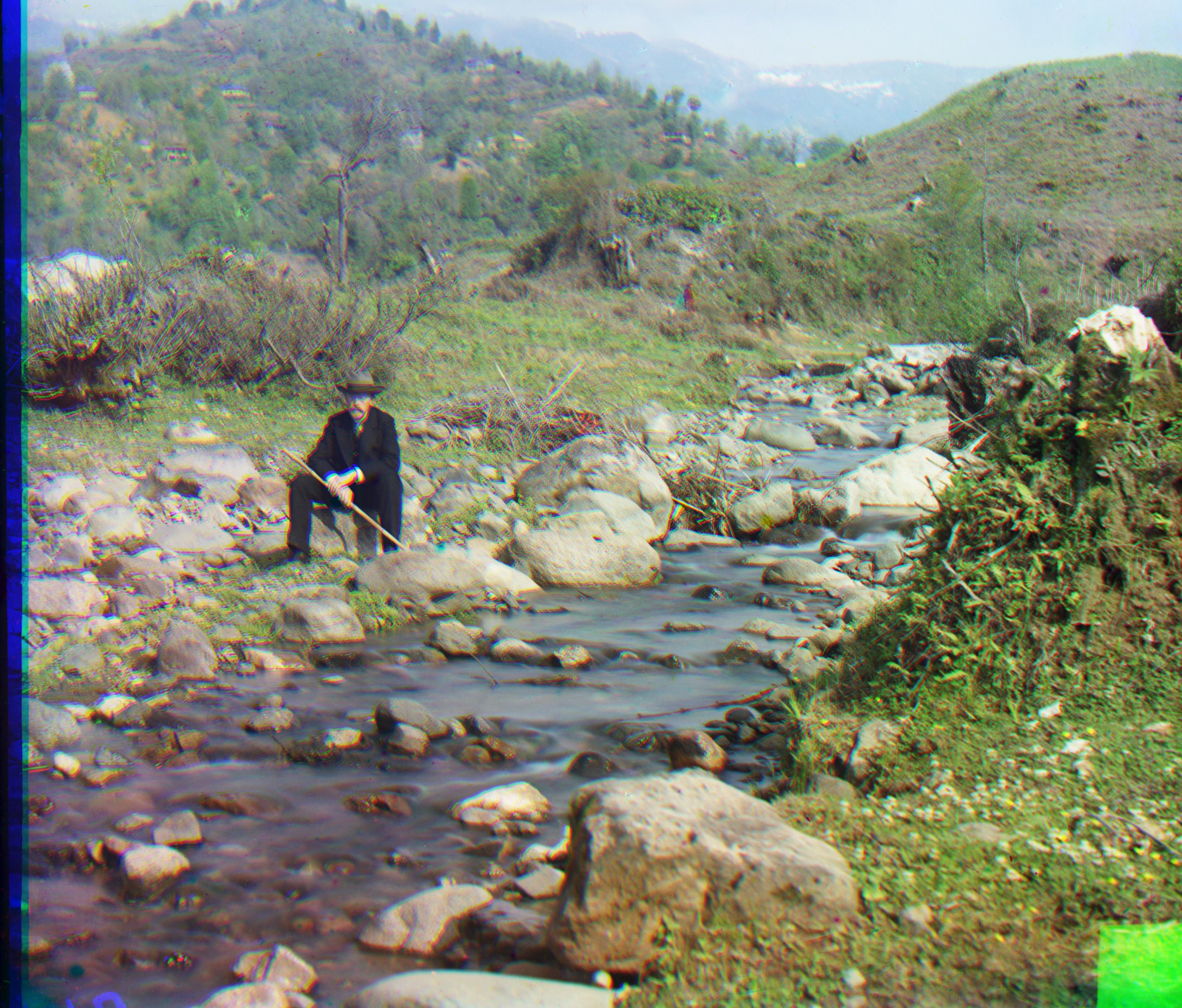
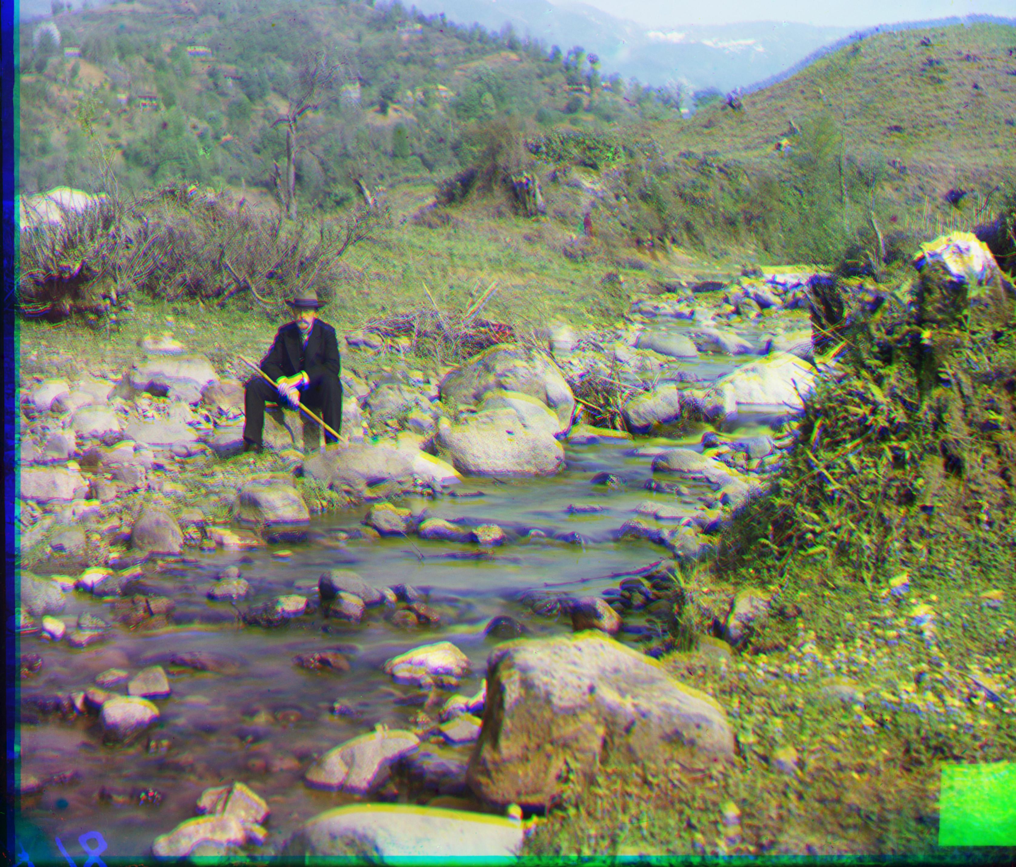
The solution I ended up finding was changing the base color channel with which to align the other two channels. On the trouble images, the blue base channel resulted in the algorithm having difficulty finding the best correction vector for the green and red color channels, but using a green base channel, the algorithm found a better correction vector the color hazing around boundaries was not longer perceivable. I outputted the correction vectors using all three color channels as base channels and my observations as to why the green color channel worked better as a base channel was because the green color channel was generally more centrally aligned in the image and the other two color channels. In other words, whereas using either blue or red color channels as base channels, the correction vectors frequently required over 100 pixels of shift in a certain direction, the green color channel typically stayed below 100 pixels of shift. Due to the smaller correction requirement necessitated by the green base channel, the pyramid search algorithm could be made more lightweight to process images faster with better results. Thus, all the images displayed on this website were generated using the green color channel. Below are some examples of trouble images produced using different base channels for alignment.
Looking at the self_portrait.tif example above, using the blue base channel resulted in a blurry image that did not have the other color channels align well. Specifically, the red color channel appears to be quite off since there are red shadows visible around borders.
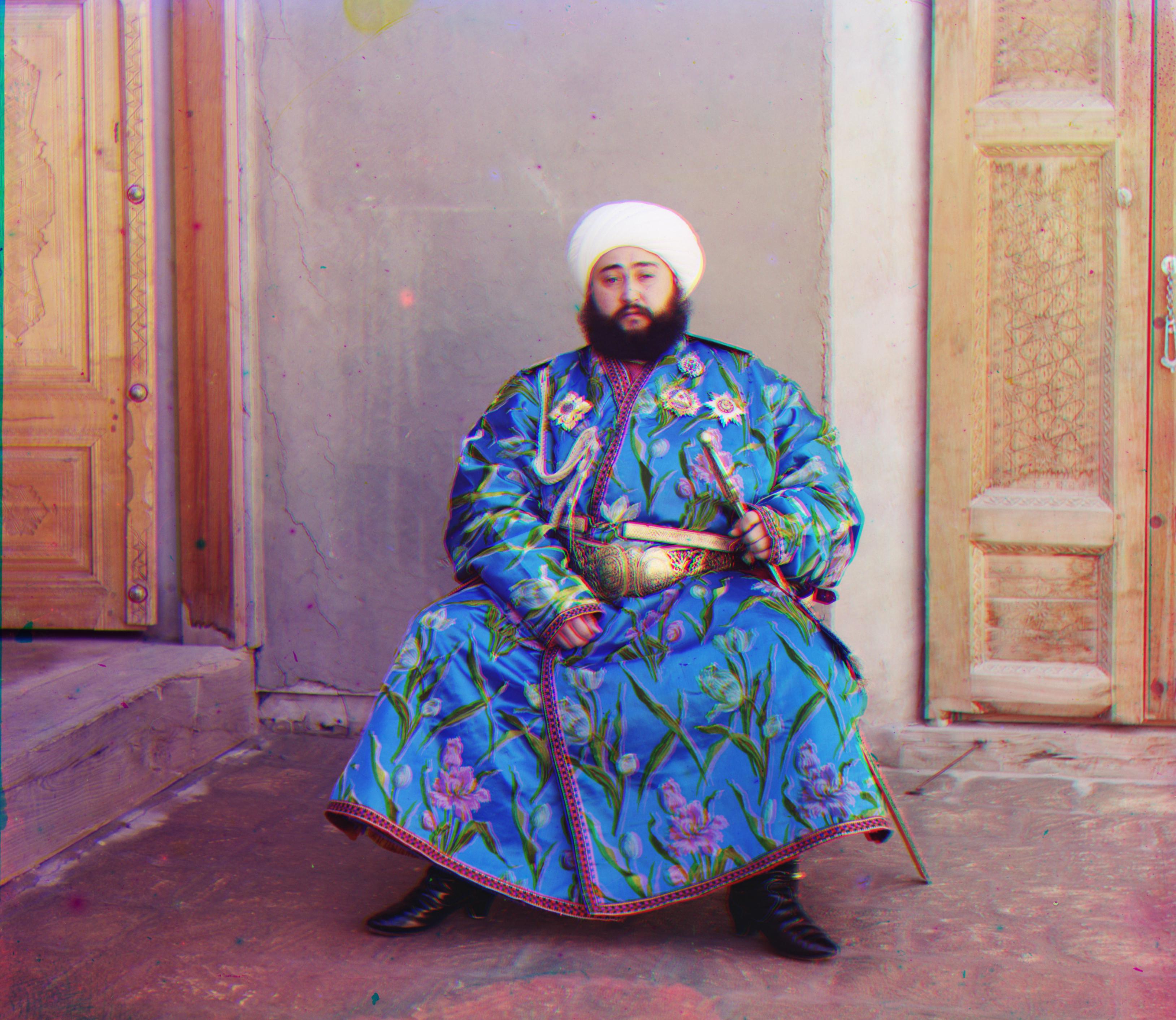
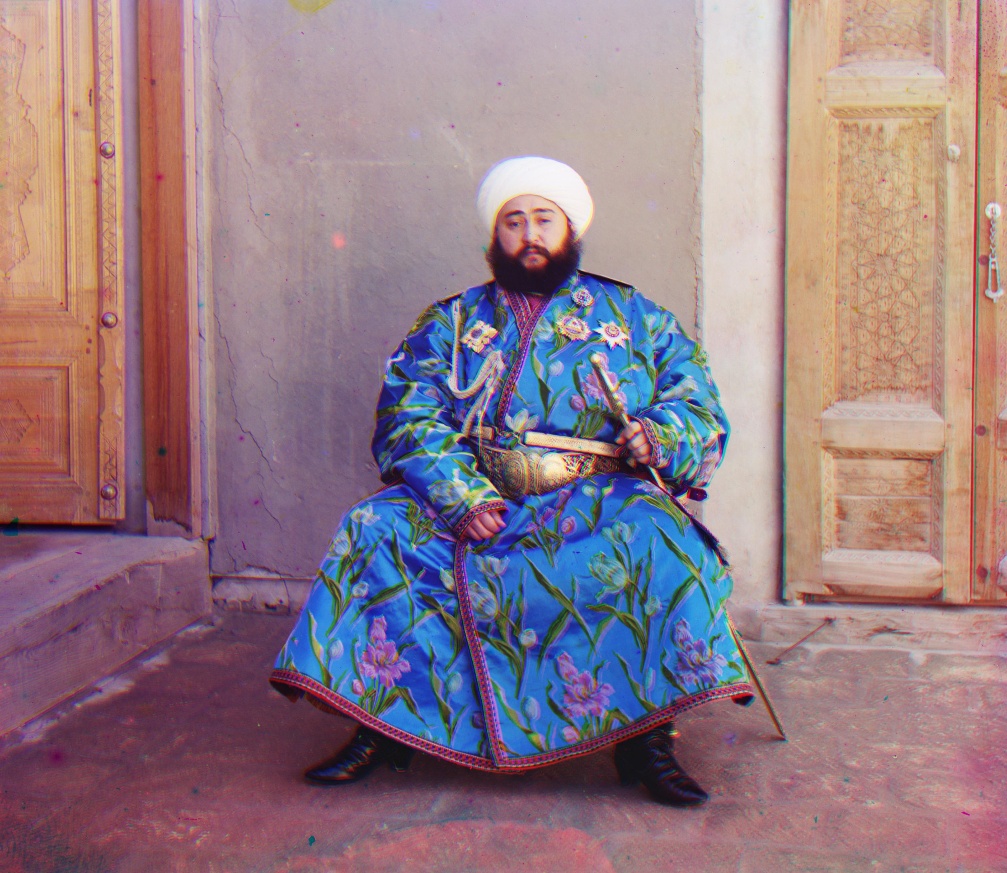
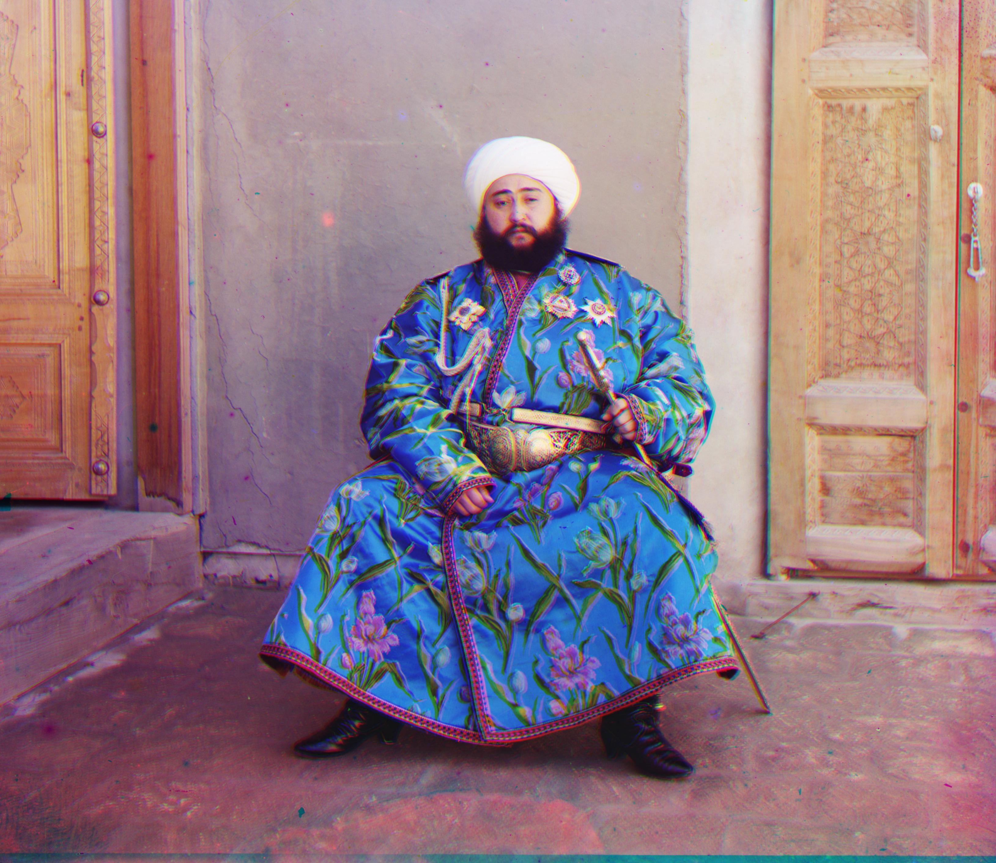
Not as noticeable but similar effect can be observed from the outputs of emir.tif with the blue base channel showing misalignment of the color channels and a blue haze around the individual in the photograph. The alignment issue is solved using a green base channel although the red base channel also does not look bad.
Since the color channels had to be aligned and shifted to match the three images and produce the final color image, the perimeter of the color images is composed of color artifacts from the color channel shifts. I realized that the severity of the artifacts was relatively the same across all images so in order to create the final color images displayed below, I applied a fixed cropping algorithm to all the color images removing 6% on each side of the image. I came to the 6% value through trial and error and it was the best value that removed most of the distracting artifacts from around the image while losing the least amount of information from the actual image.
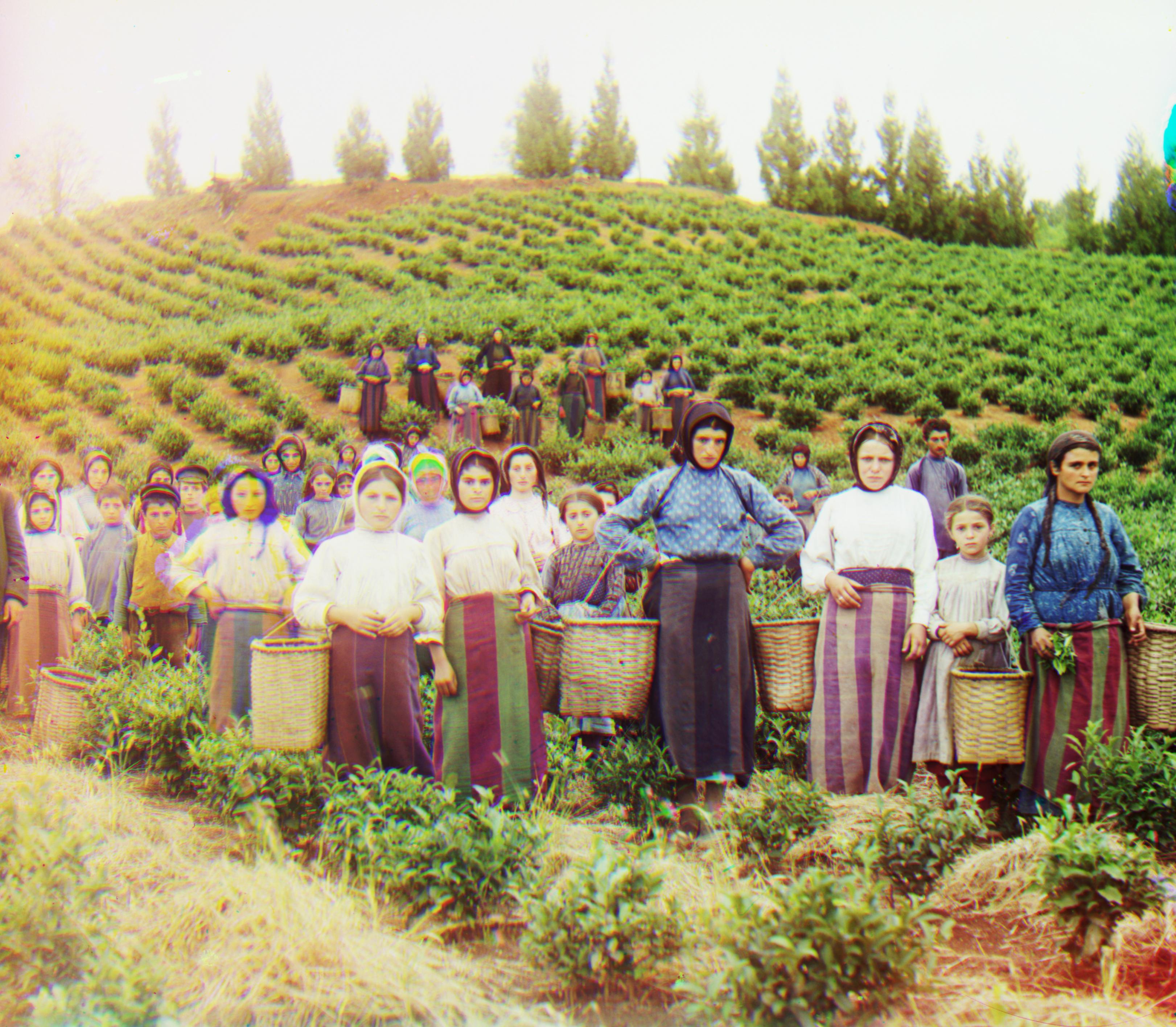
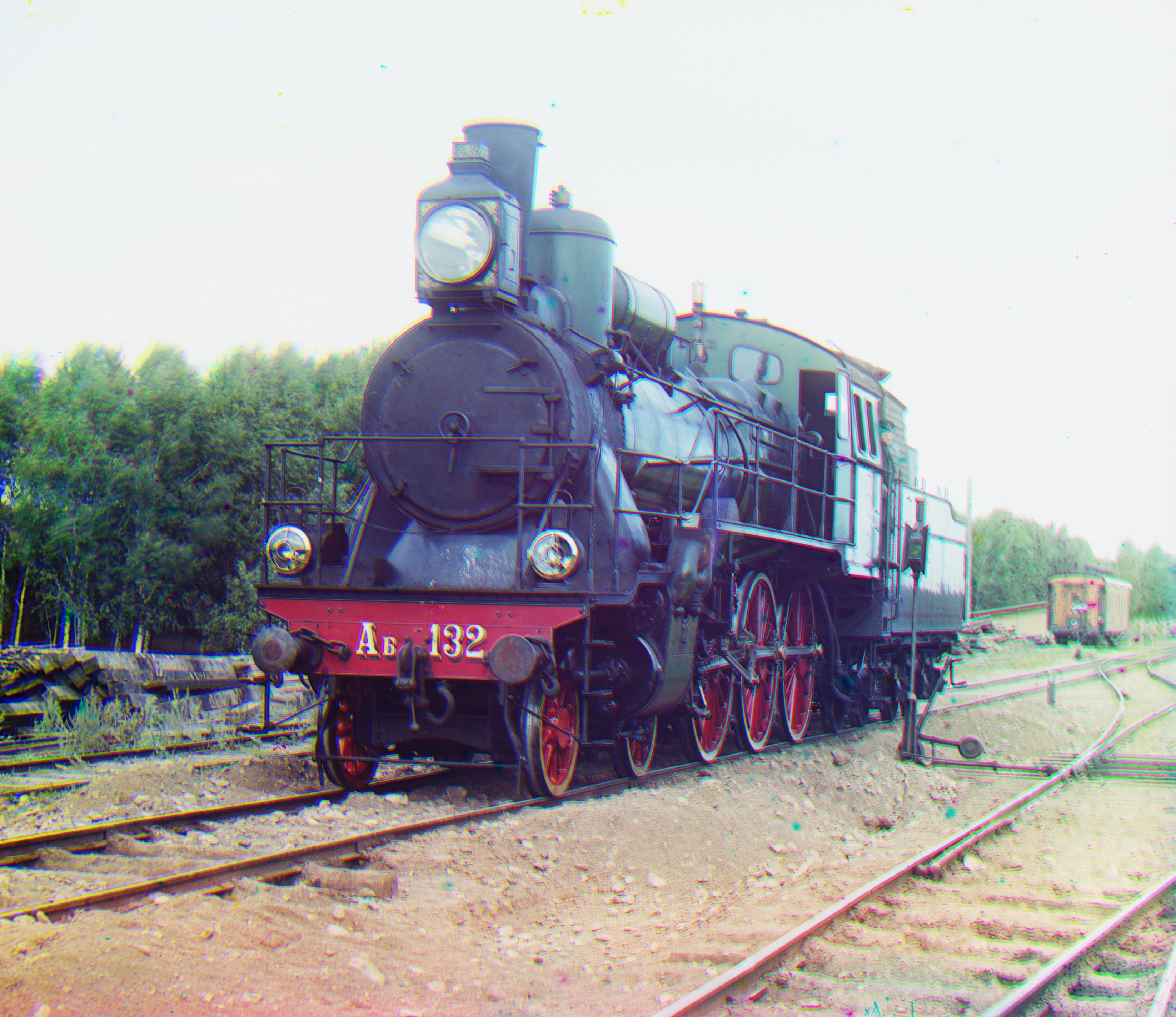
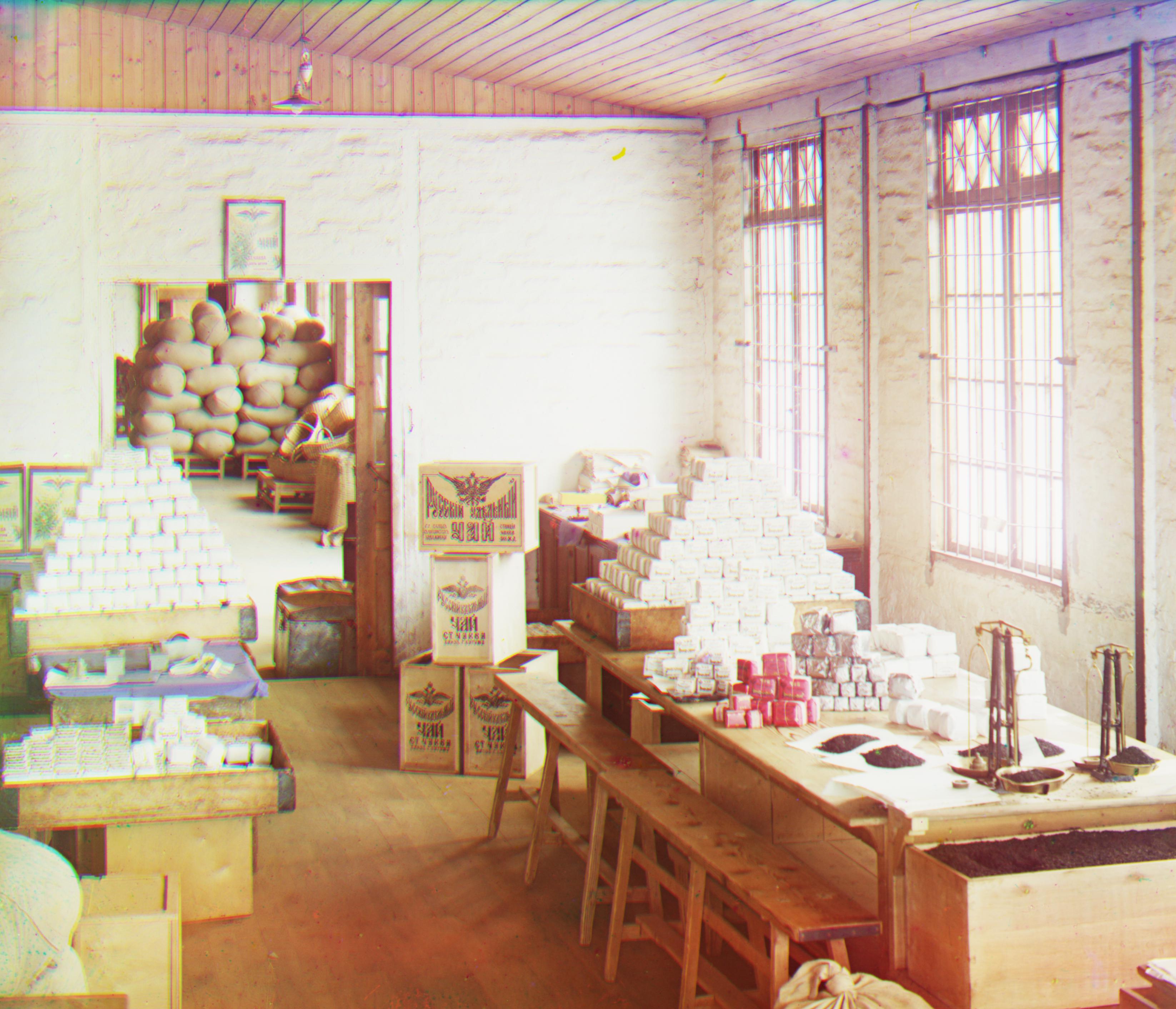
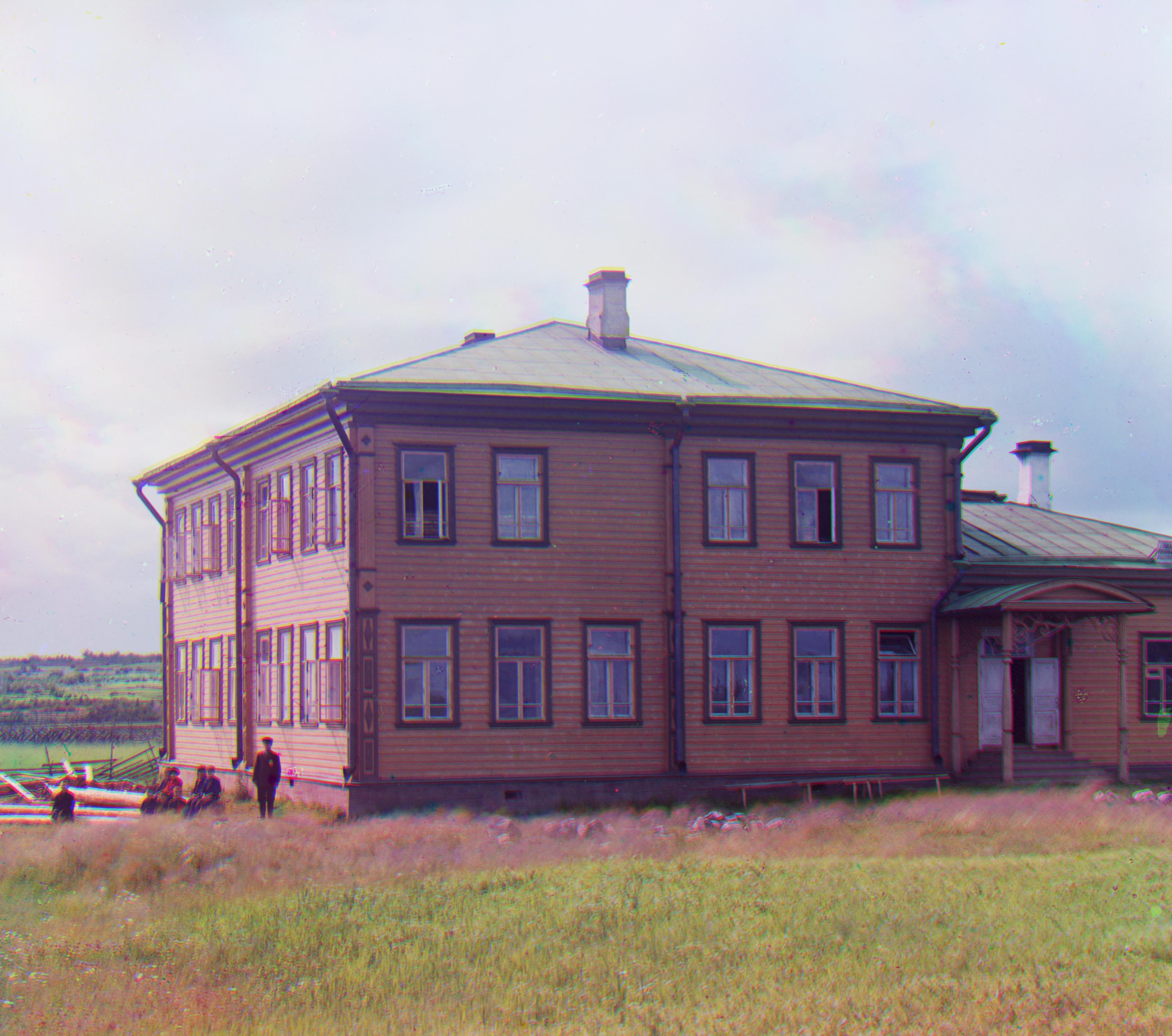
Below are all the generated images from the provided negatives.
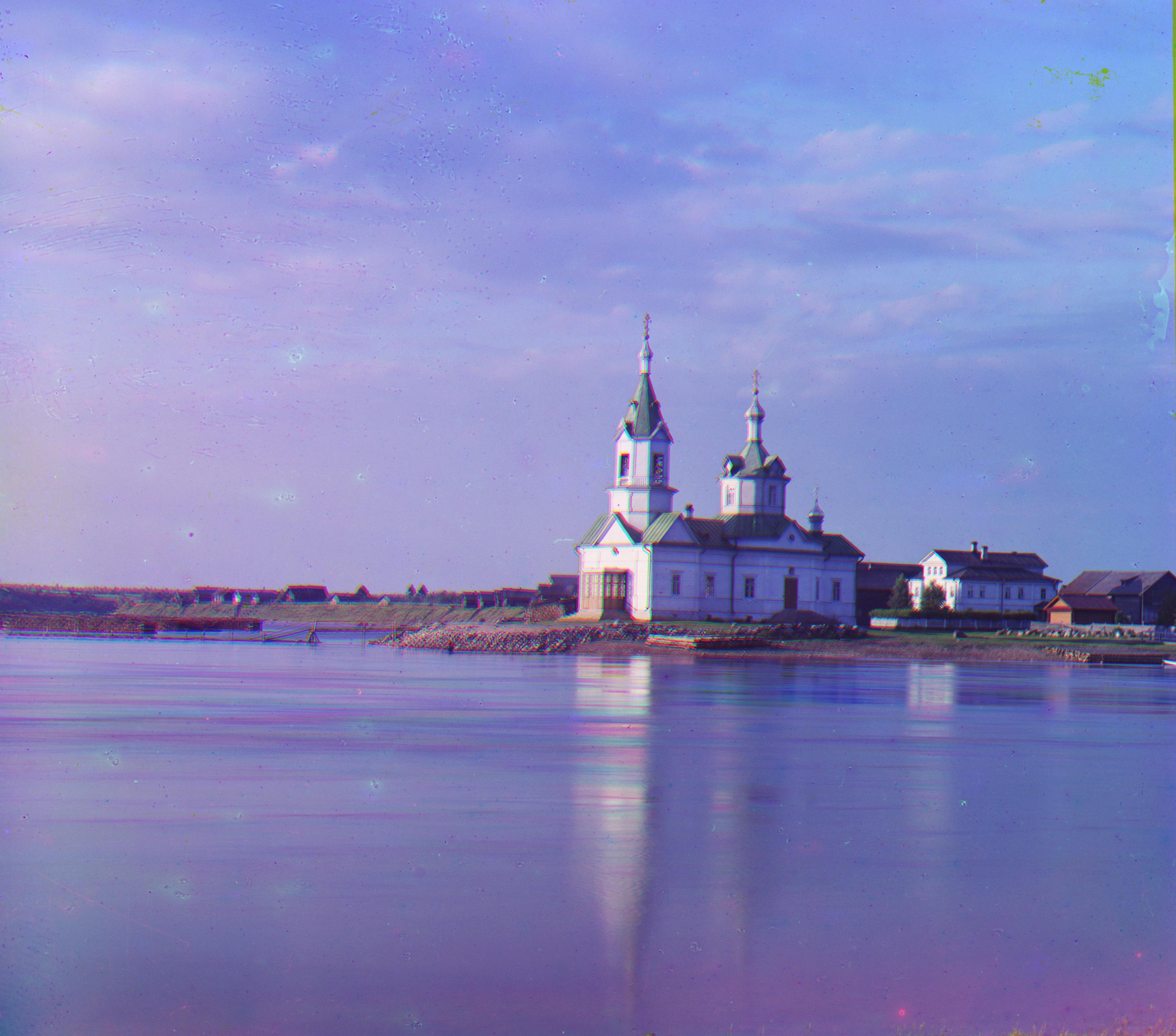
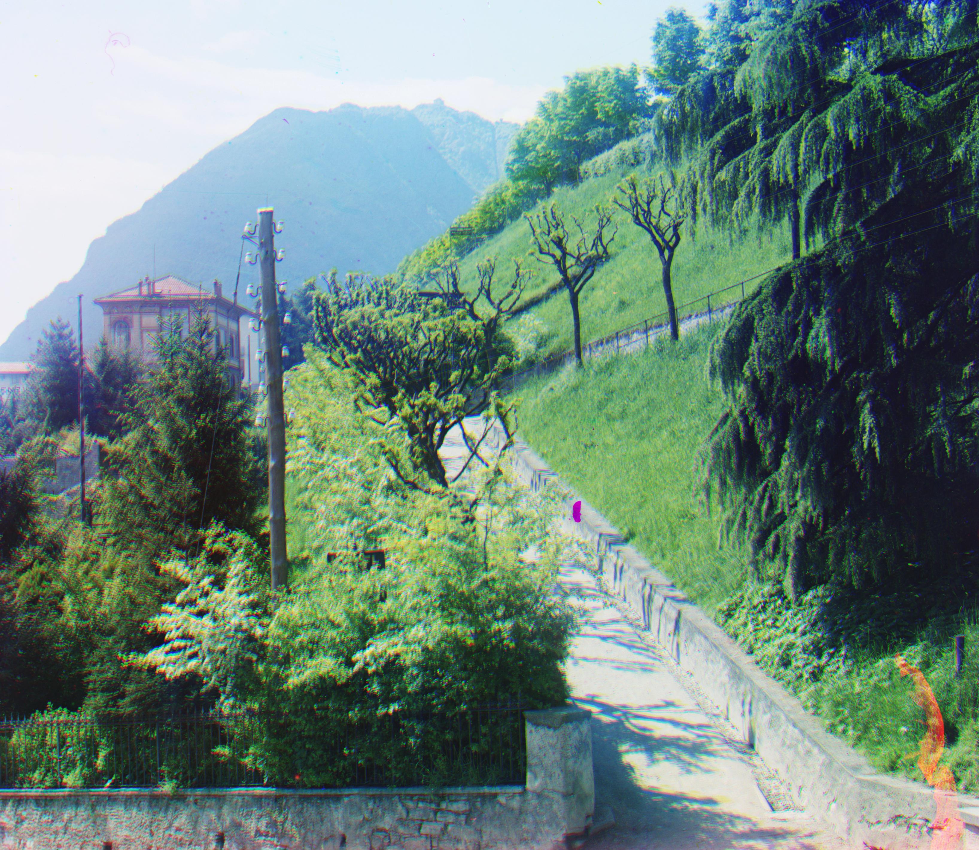
Below are three generated images from negatives that I found online from the Library of Congress.
This section includes the outputted correction vectors using all three color channels as base channels. Images whose negatives were provided as .jpg were generated using exhaustive search and images whose negatives were provided as .tif were generated using pyramid search.
Blue Base Channel |
||
|---|---|---|
| Image Name | Green Channel Correction (x,y) | Red Channel Correction (x,y) |
| cathedral.jpg | (2, 5) | (3, 12) |
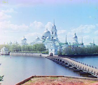
| church.tif | (8, 29) | (-9, 63) |
| emir.tif | (29, 53) | (54, 107) |
| harvesters.tif | (21, 65) | (19, 129) |
| icon.tif | (21, 45) | (27, 90) |
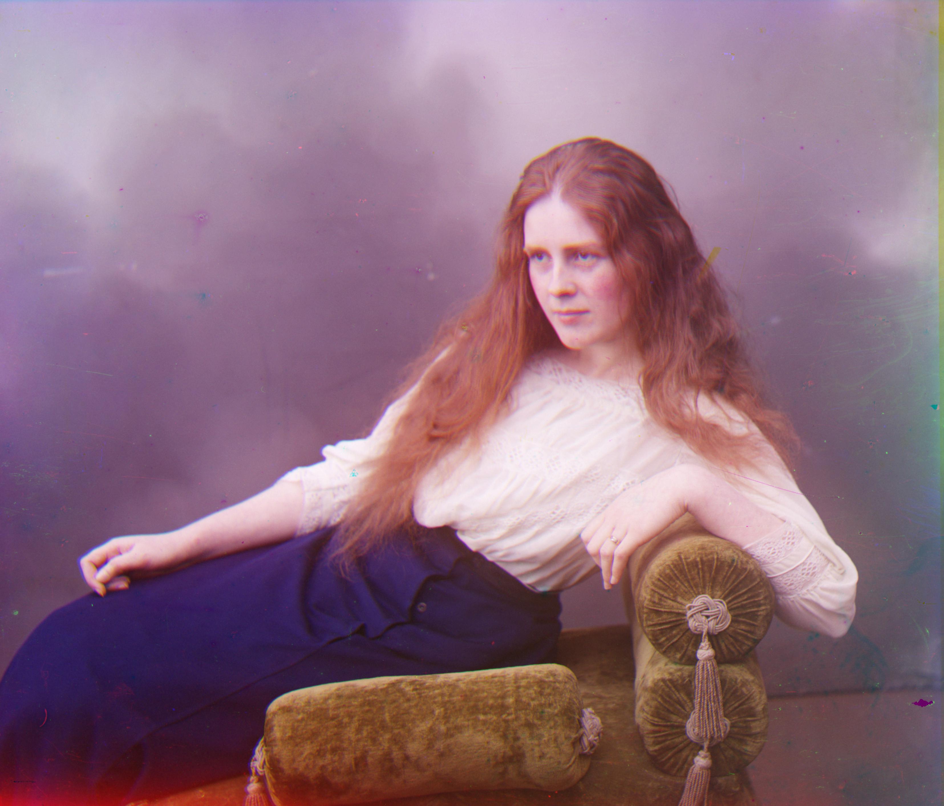
| lady.tif | (13, 55) | (7, 117) |
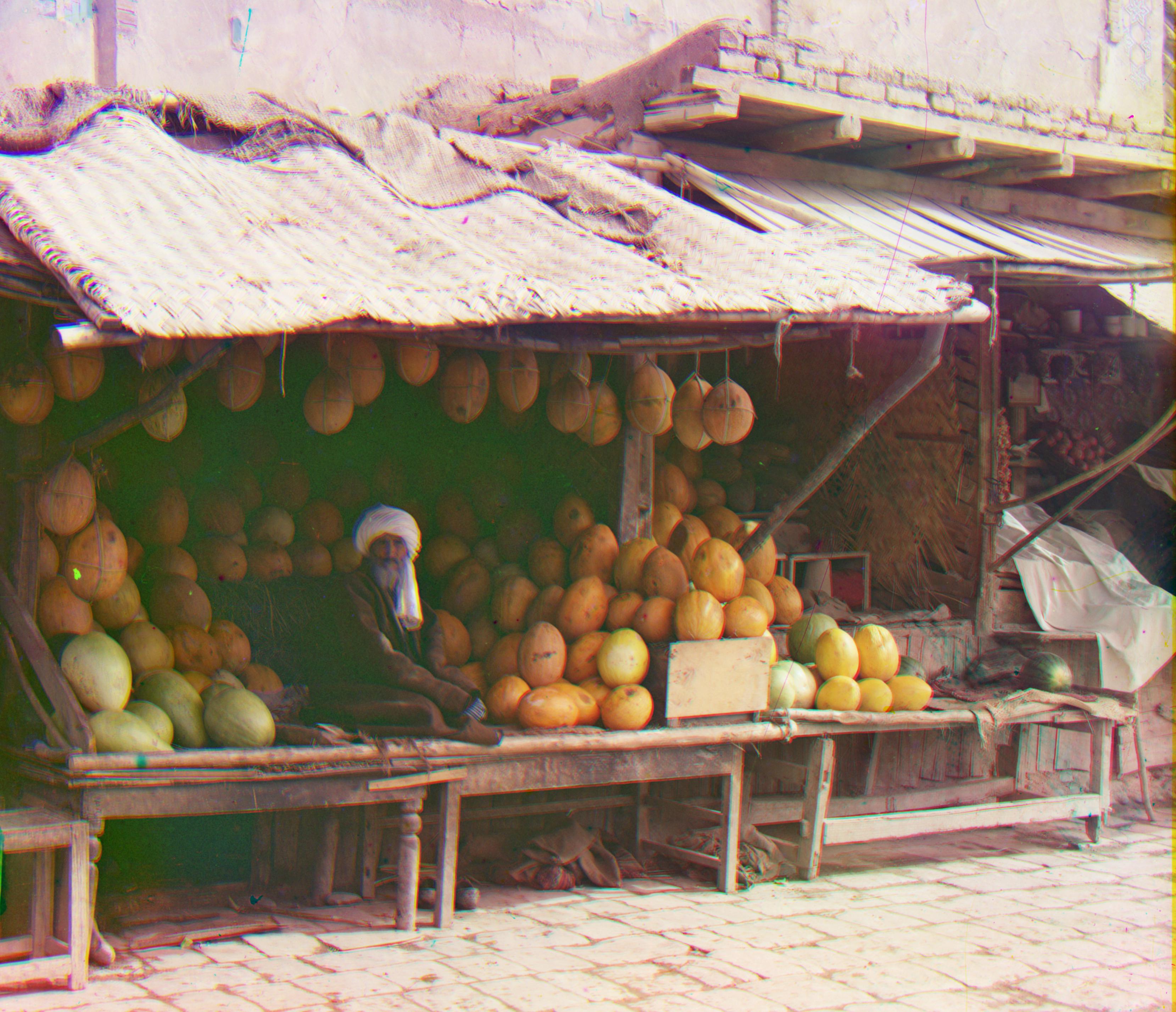
| melons.tif | (12, 87) | (15, 155) |
| monastery.jpg | (2, -3) | (2, 3) |
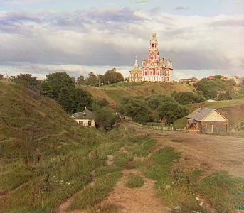
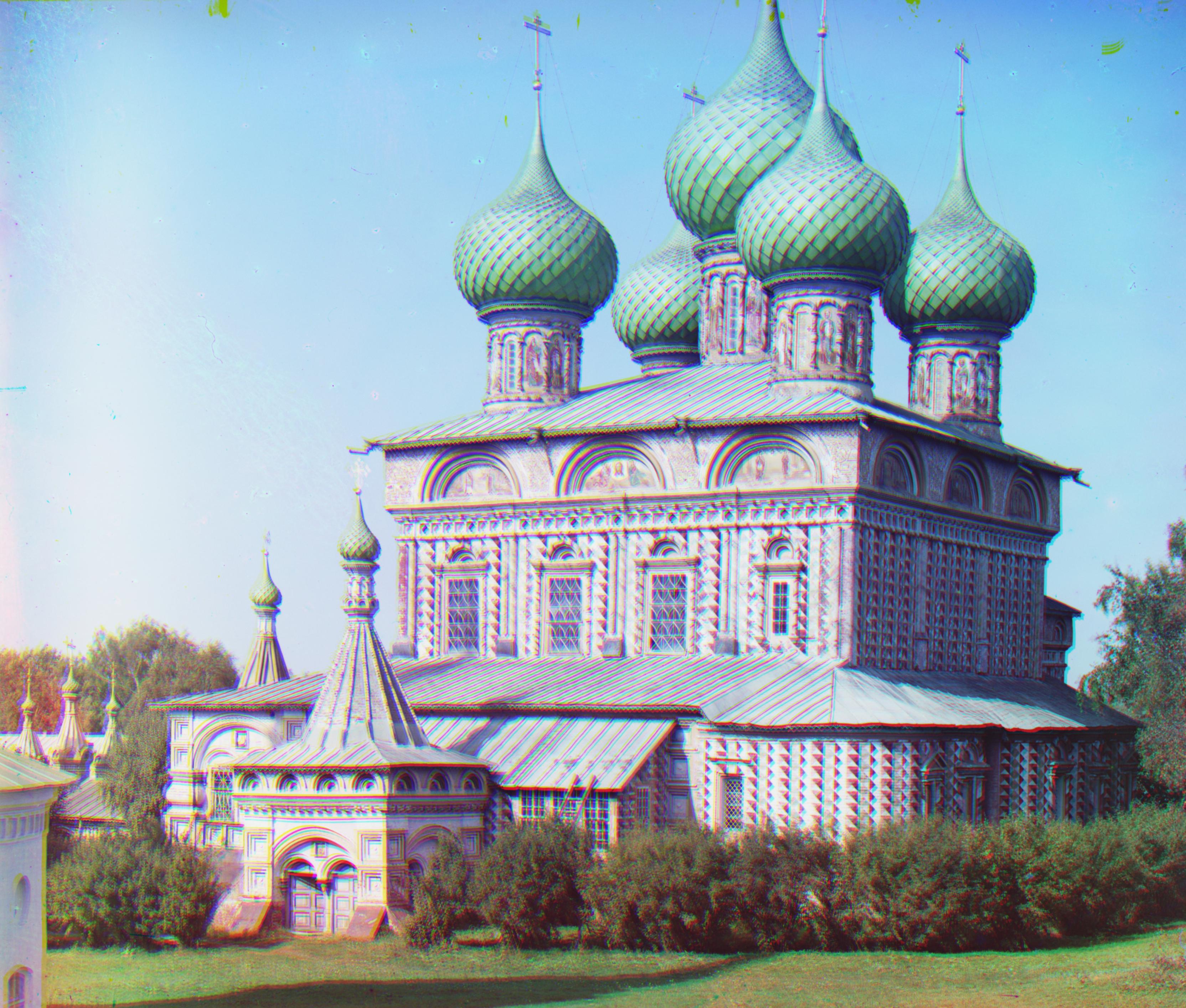
| onion_church.tif | (31, 57) | (41, 113) |
| self_portrait.tif | (33, 83) | (37, 155) |
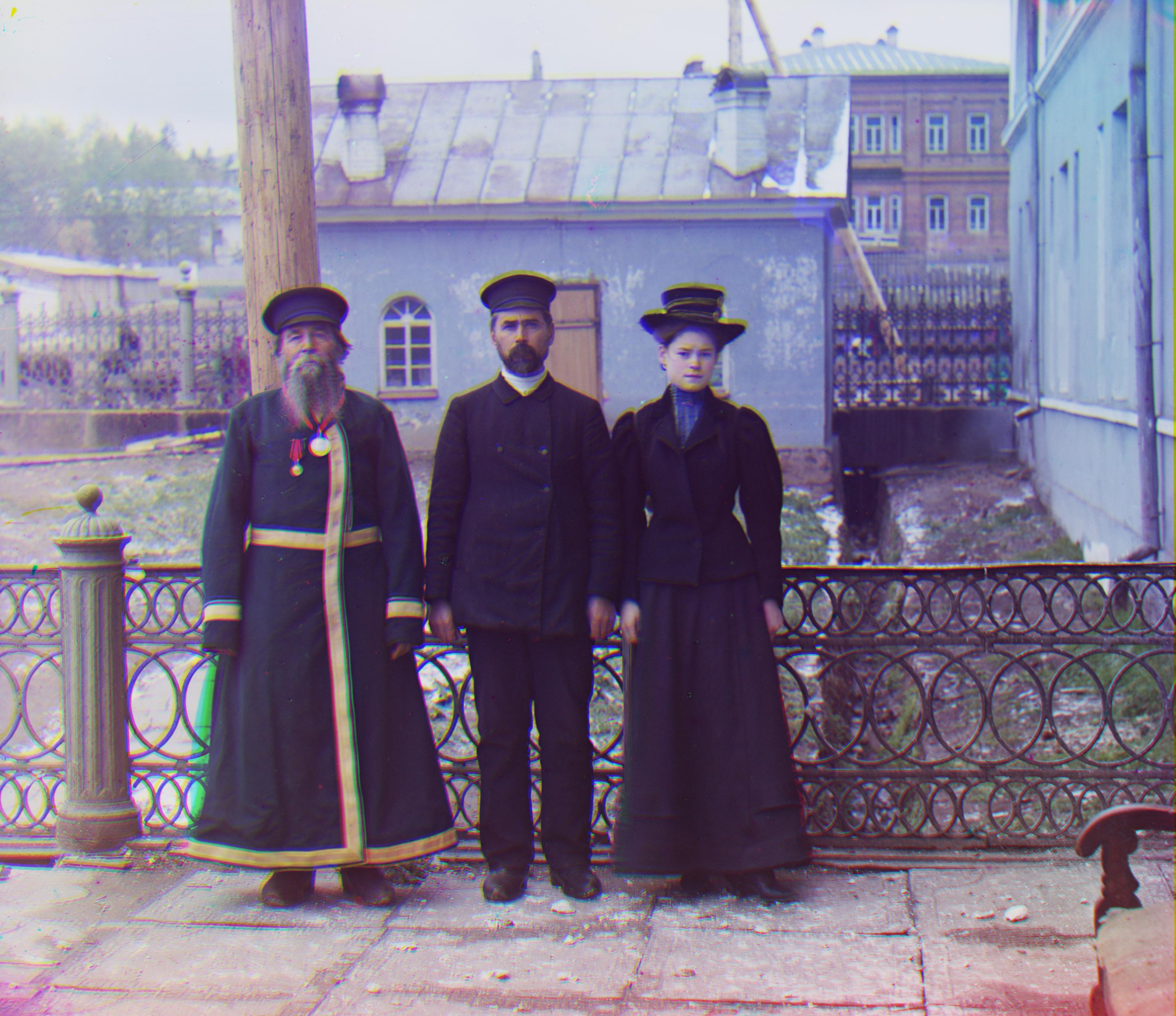
| three_generations.tif | (19, 59) | (15, 117) |
| tobolsk.jpg | (3, 3) | (3, 6) |
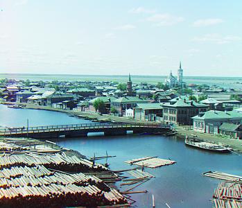
| train.tif | (9, 47) | (32, 93) |
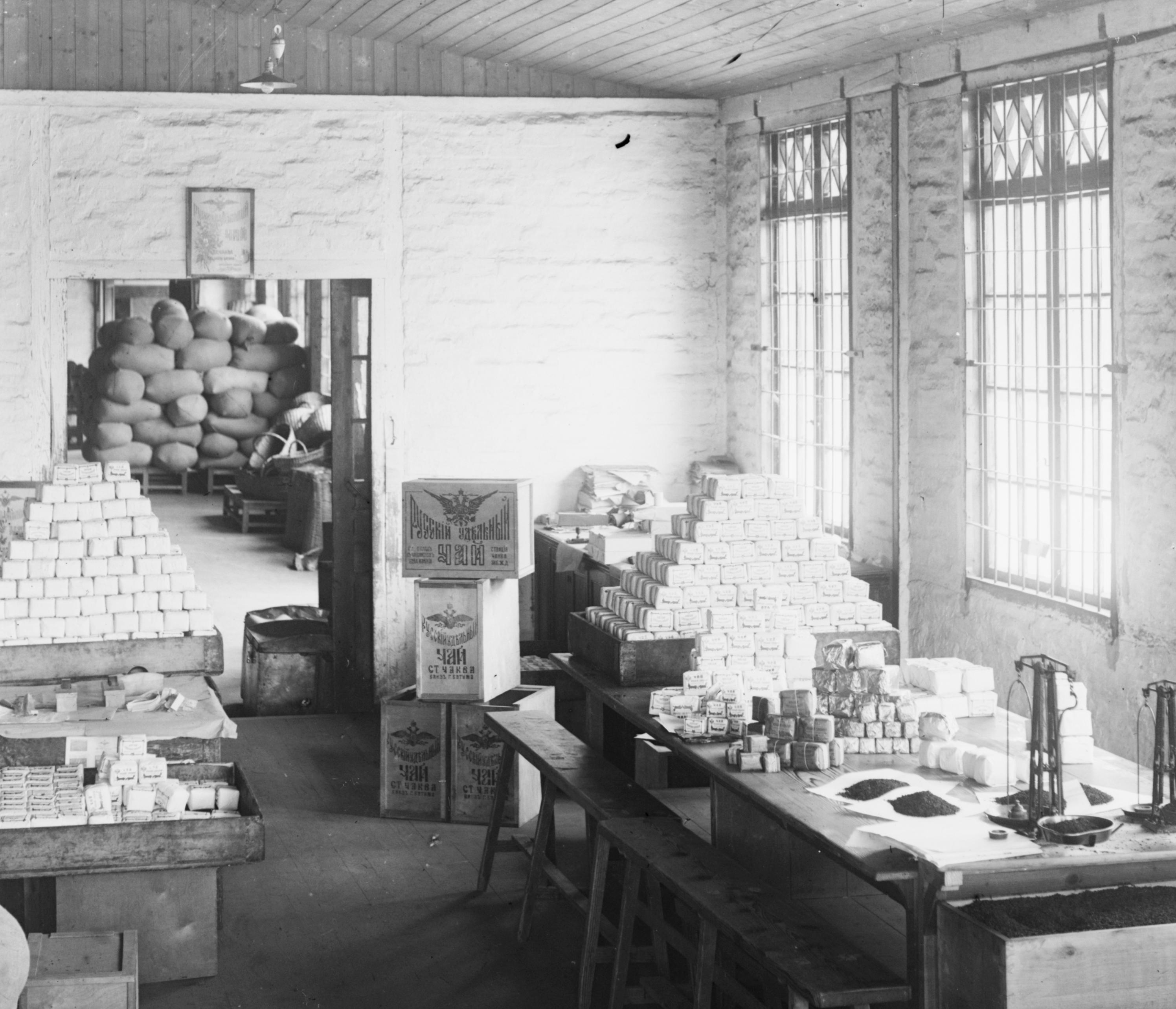
| workshop.tif | (2, 57) | (-17, 109) |
| school.tif | (15, 31) | (15, 67) |
| capri.tif | (-21, 33) | (-34, 69) |
| coal_furnace.tif | (-4, 23) | (-8, 99) |
Green Base Channel |
||
|---|---|---|
| Image Name | Blue Channel Correction (x,y) | Red Channel Correction (x,y) |
| cathedral.jpg | (-2, -5) | (1, 7) |
| church.tif | (-8, -29) | (-13, 39) |
| emir.tif | (-29, -53) | (23, 61) |
| harvesters.tif | (-21, -65) | (-2, 69) |
| icon.tif | (-21, -45) | (11, 53) |
| lady.tif | (-13, -55) | (4, 65) |
| melons.tif | (-12, -87) | (8, 101) |
| monastery.jpg | (-2, 3) | (1, 6) |
| onion_church.tif | (-31, -57) | (15, 63) |
| self_portrait.tif | (-33, -83) | (13, 103) |
| three_generations.tif | (-19, -59) | (-4, 63) |
| tobolsk.jpg | (-3, -3) | (1, 4) |
| train.tif | (-9, -47) | (31, 49) |
| workshop.tif | (-2, -57) | (-15, 57) |
| school.tif | (-15, -31) | (0, 41) |
| capri.tif | (21, -33) | (-18, 43) |
| coal_furnace.tif | (4, -23) | (-4, 81) |
Red Base Channel |
||
|---|---|---|
| Image Name | Green Channel Correction (x,y) | Blue Channel Correction (x,y) |
| cathedral.jpg | (-1, -7) | (-3, -12) |
| church.tif | (9, -63) | (13, -39) |
| emir.tif | (-23, -61) | (-54, -107) |
| harvesters.tif | (2, -69) | (-19, -129) |
| icon.tif | (-11, -53) | (-27, -90) |
| lady.tif | (-4, -65) | (-7, -117) |
| melons.tif | (-8, -101) | (-15, -155) |
| monastery.jpg | (-1, -6) | (-2, -3) |
| onion_church.tif | (-15, -63) | (-41, -113) |
| self_portrait.tif | (-13, -103) | (-37, -155) |
| three_generations.tif | (4, -63) | (-15, -117) |
| tobolsk.jpg | (-1, -4) | (-3, -6) |
| train.tif | (-31, -49) | (-32, -93) |
| workshop.tif | (15, -57) | (17, -109) |
| school.tif | (0, -41) | (-15, -67) |
| capri.tif | (18, -43) | (34, -69) |
| coal_furnace.tif | (4, -81) | (8, -99) |