Project Overview: Abel Yagubyan
Introduction
"Sergey Mikhaylovich Prokudin-Gorsky (August 18, 1863 - September 27, 1944) was a chemist and photographer of the Russian Empire. He is best known for his pioneering work in colour photography and his effort to document early 20th-century Russia." [via Wikipedia]"Using a railroad-car darkroom provided by Tsar Nicholas II, Prokudin-Gorsky traveled the Russian Empire from around 1909 to 1915 using his three-image colour photography to record its many aspects. While some of his negatives were lost, the majority ended up in the U.S. Library of Congress after his death. Starting in 2000, the negatives were digitised and the colour triples for each subject digitally combined to produce hundreds of high-quality colour images of Russia and its neighbors from over a century ago."[via Wikipedia]
"The goal of this assignment is to take the digitized Prokudin-Gorskii glass plate images and, using image processing techniques, automatically produce a color image with as few visual artifacts as possible. In order to do this, I extracted the three color channel images, placed them on top of each other, and aligned them so that they form a single RGB color image."[via 194-26 Website]
Configurations
Before going into the implemented processing techniques used for the given set of images, I'll just go over some of the features that I implemented to optimize the looks of the images.SSD vs NCC
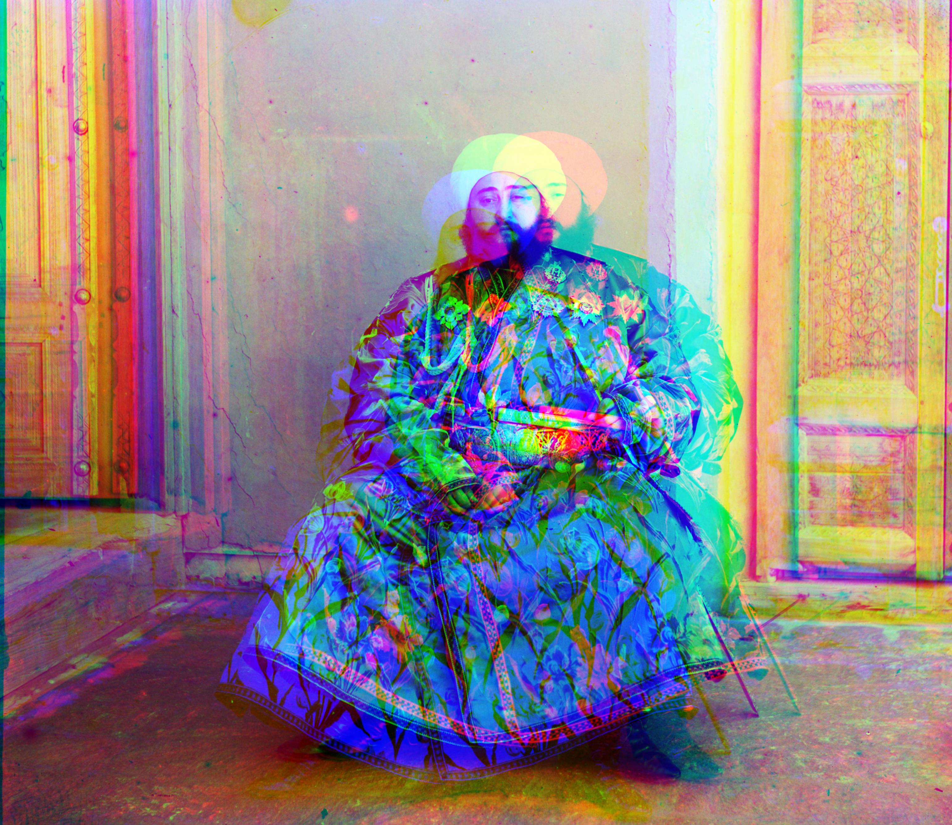
Before being able to actually complete the image processing, the Sum of Squared Differences (SSD, distance which is simply sum(sum((image1-image2).^2))) processing of the image pixels must be compared with the cross-correlation (NCC) (which is simply a dot product between two normalized vectors: (image1./||image1|| and image2./||image2||)) in order to get the best possible image results. As displayed below, the SSD image (left) on theemir.tif image looks much better than the NCC image (right). Due to this, my implementation for all of the image processing techniques uses SSD as the base image matching metric.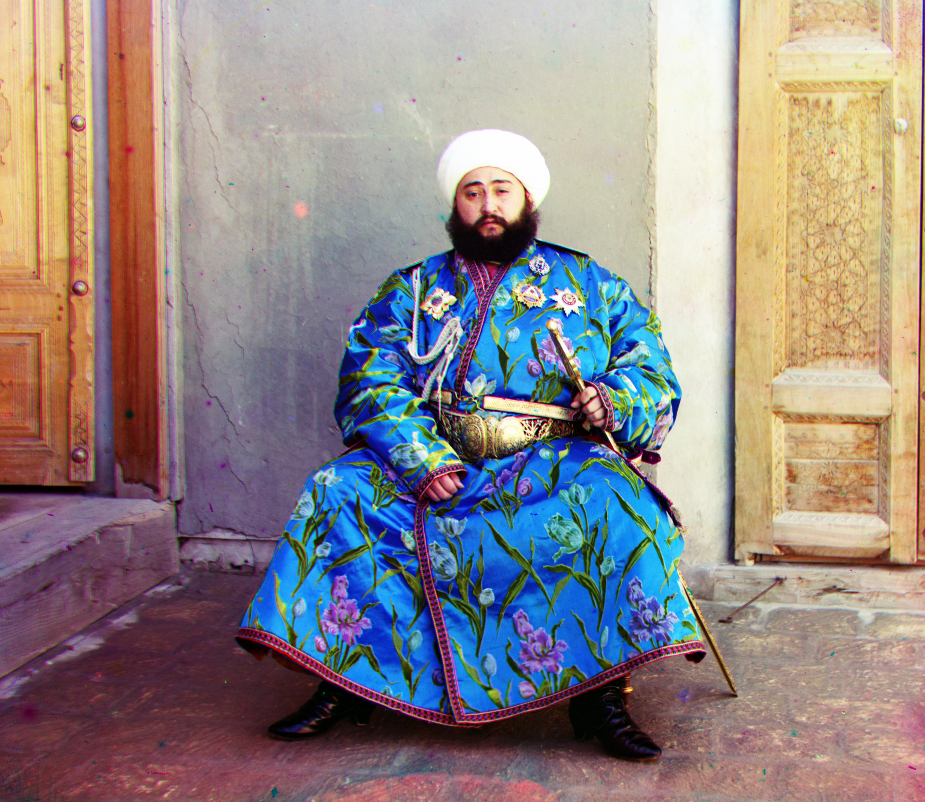
Base Channel
Interestingly enough, choosing the base channel drastically changes the results of the images and how processing should be handled in the latter stages of the processing. As it can be seen, using the base channel resulted in an image in the middle (Green Channel) that is much better than the images on the far-left (Red Base Channel) and the far-right (Blue Base Channel). Due to this, all of the images use a base channel of Green to produce the most perfect images.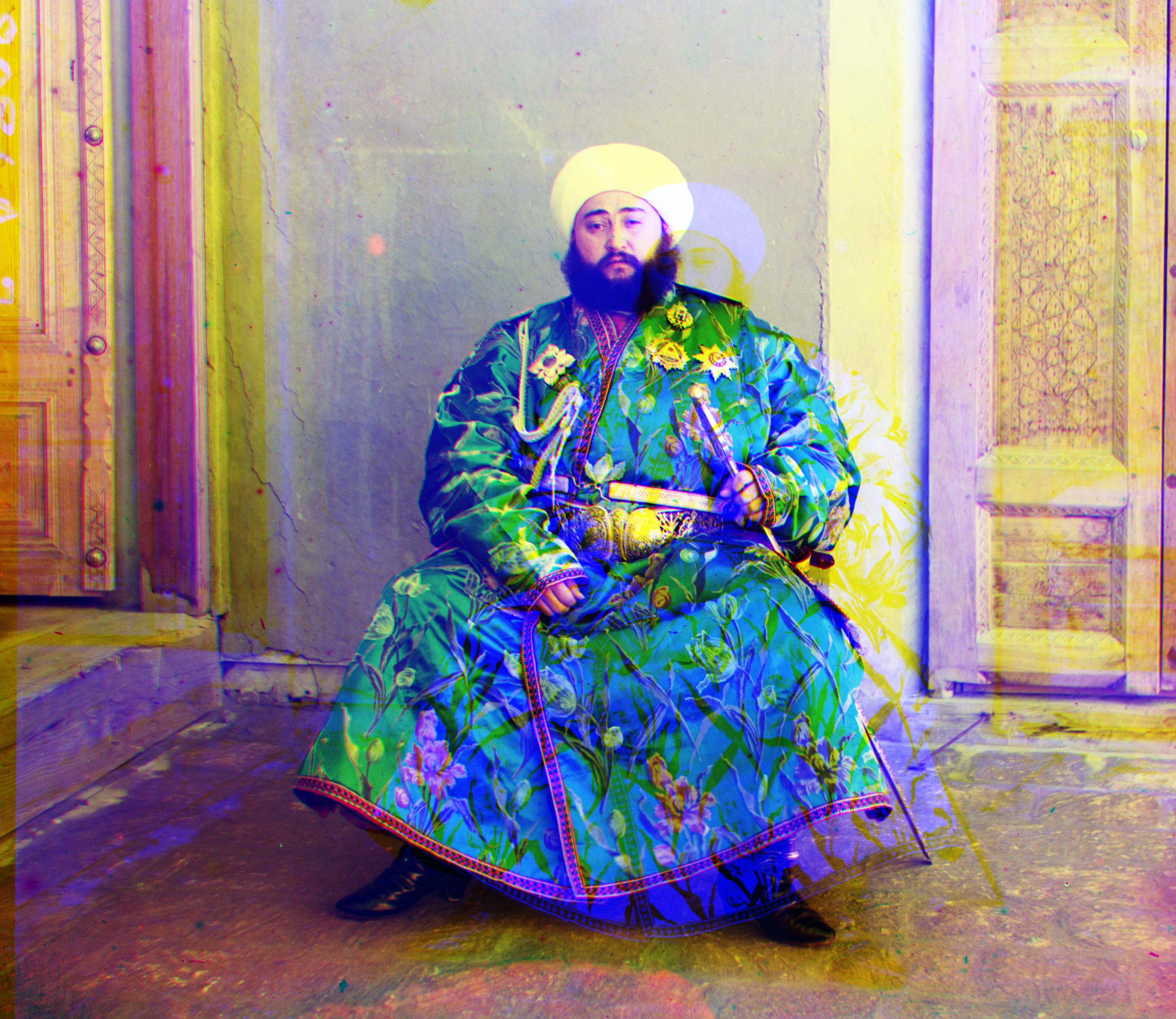

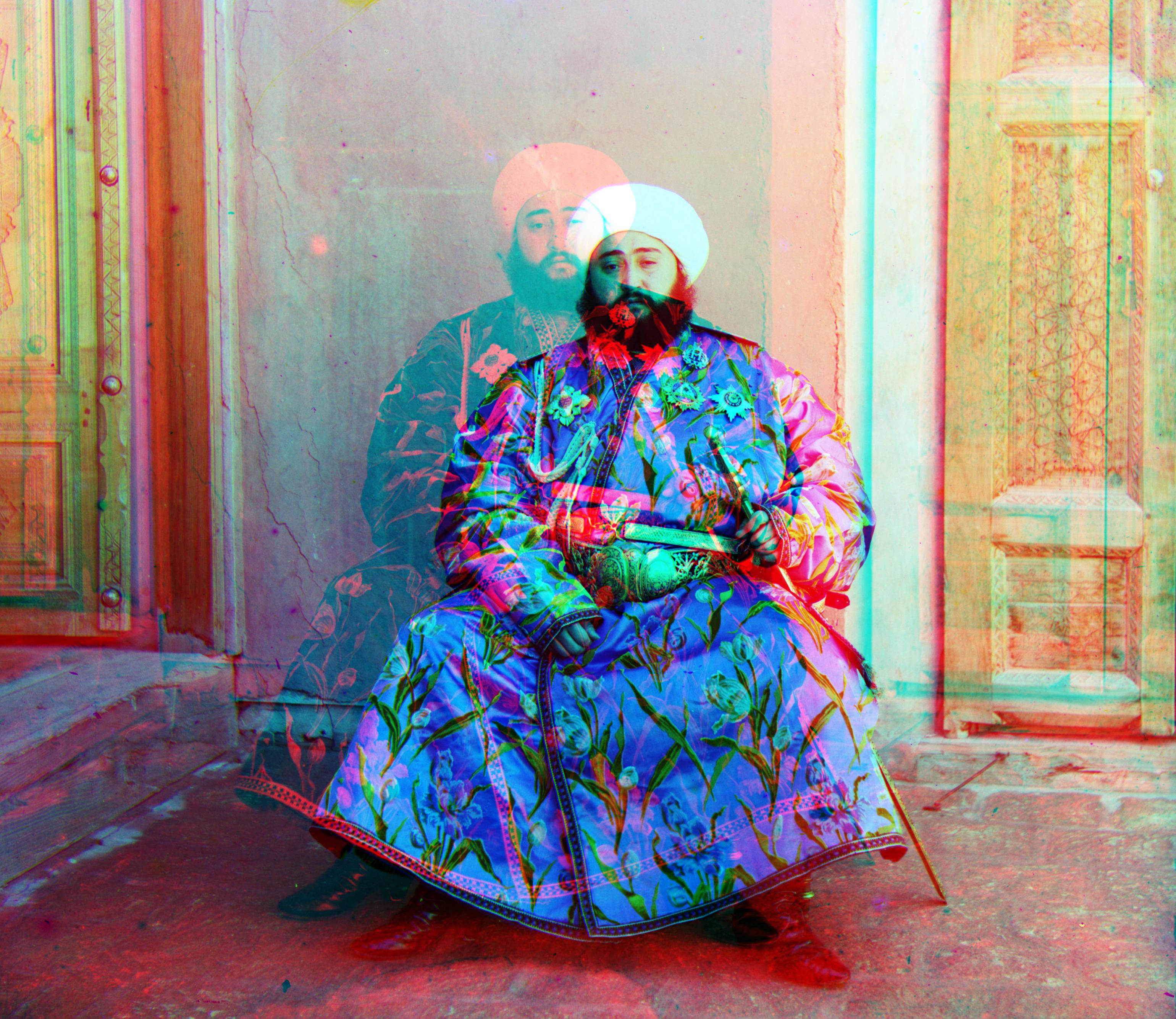
Image Cropping
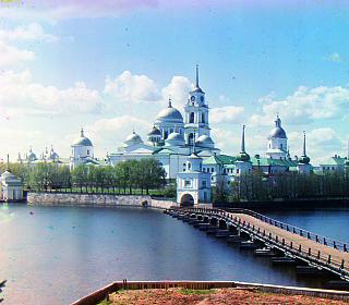
As you might've already noticed, the images above look too good to be true! Well, since the image was built by combining three image filters to make a single one (it was the early 1900s after all), the borders should have misaligned colored stripes and dark-ish boundaries. Well that was certainly the case with my images too, but what I went ahead and did was to crop a fixed amount of ~8.3% of the image from all sides of all the images. Luckily enough, all of the images look great with this amount (although I would love to work on auto-cropping, but life happened :( ). In the images below, you can see how the uncropped images looked (left) and how the cropped ones looked (right).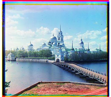
Initial Image Processing
Now that we have gone through the configurations, we can go ahead and talk about the initial processing done to all the images. Before anything, we must split the input image into three filters (B,G, and R), which was easily done by splitting the input image into 3 equivalent parts. After having done that, I create a copied image which I used to crop out approximately 20% from each side of the filter images to use as an input vector into our exhaustive searches and image pyramids, as described later on. This was done to optimize our image on the central pixels of the image to get the best possible displacement alignments on the images. After having done that, we are ready to process our copied and cropped out images to get the displacement values for the filters!Single-Scale Implementation
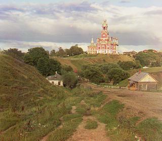
For lower-res images, we will use the exhaustive search method to iterate through the image pixels (of x and y values between [-15,15]) and use our image alignment scoring techniques (as described above) to retrieve the best possible displacement results for lower-res images, which were of .JPG type. You can see a few examples of the resulting images below (some examples include: Monastery, Cathedral, etc.).Multi-Scale Implementation
Now that we are beginning to deal with super-large input images of .TIF type, exhaustive search will drastically increase our runtime to find the displacement values for the images. To solve this issue, we will go ahead and use pyramid image-alignment to get these values, which essentially aligns high resolution images efficiently by downscaling them by a preset scaling factor multiple times. The algorithm uses the best displacement values from the lower res level images retrieved using the exhaustive search to then enact the same action of offseting the values to the larger res level images. However, one caviat with this approach was that the exhaustive search would still have to go through 900 (30*30) possible X and Y combinations of displacement values for every single possible image. This issue actually caused my runtime to be approximately 40s for larger-res images. Luckily though, since we begin to deal with low-res images first (and recursively go back up), we can decrease our offset limit values to [-5,5] (100 combinations) to get a much better runtime of ~4s. If need be, the scaling factor that I used for my images was 5.Finalizing Image Processing
After getting the X and Y displacement values, we usenp.roll to shift our (original, non-cropped) Red and Blue image vectors by these values to perfectly align our filters. After having done this, we crop ~8.3% of the image from each side (as mentioned previously) to get rid of the ugly borders. We then save these images as JPG type images and finish the process!
Fails!
Although the results turned out to look great (thankfully!), I attempted to work on Canny Edge detection techniques to automatically detect the edges/borders of the images to be cropped (instead of the meh-approach of fixed ~8.3% cropping of the borders of the images). Unfortunately, it completely failed and I was not able to get anything interesting from it. Luckily though, I was able to get auto-contrasting to work!Bells & Whistles (EC) - Auto Contrasting
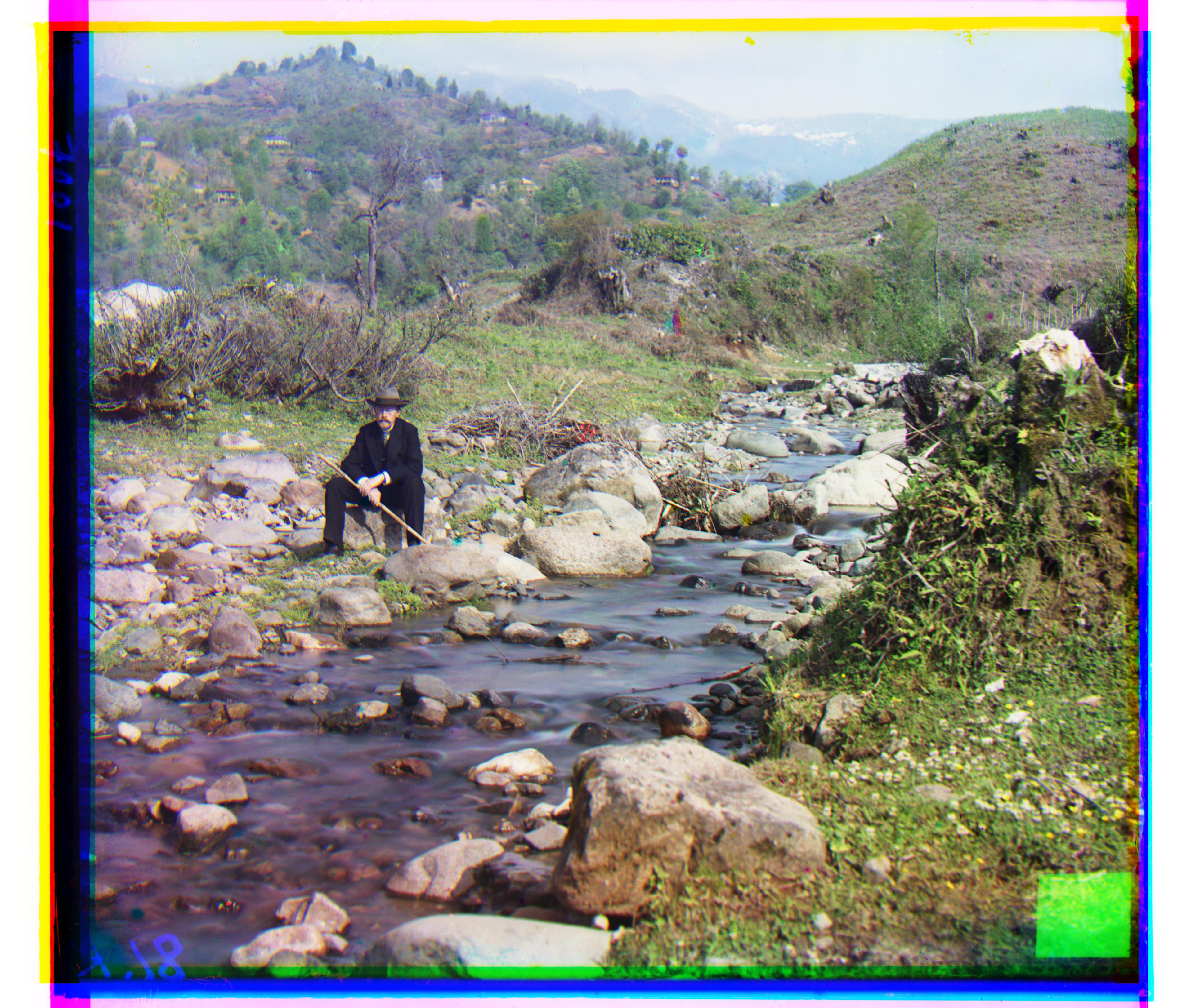
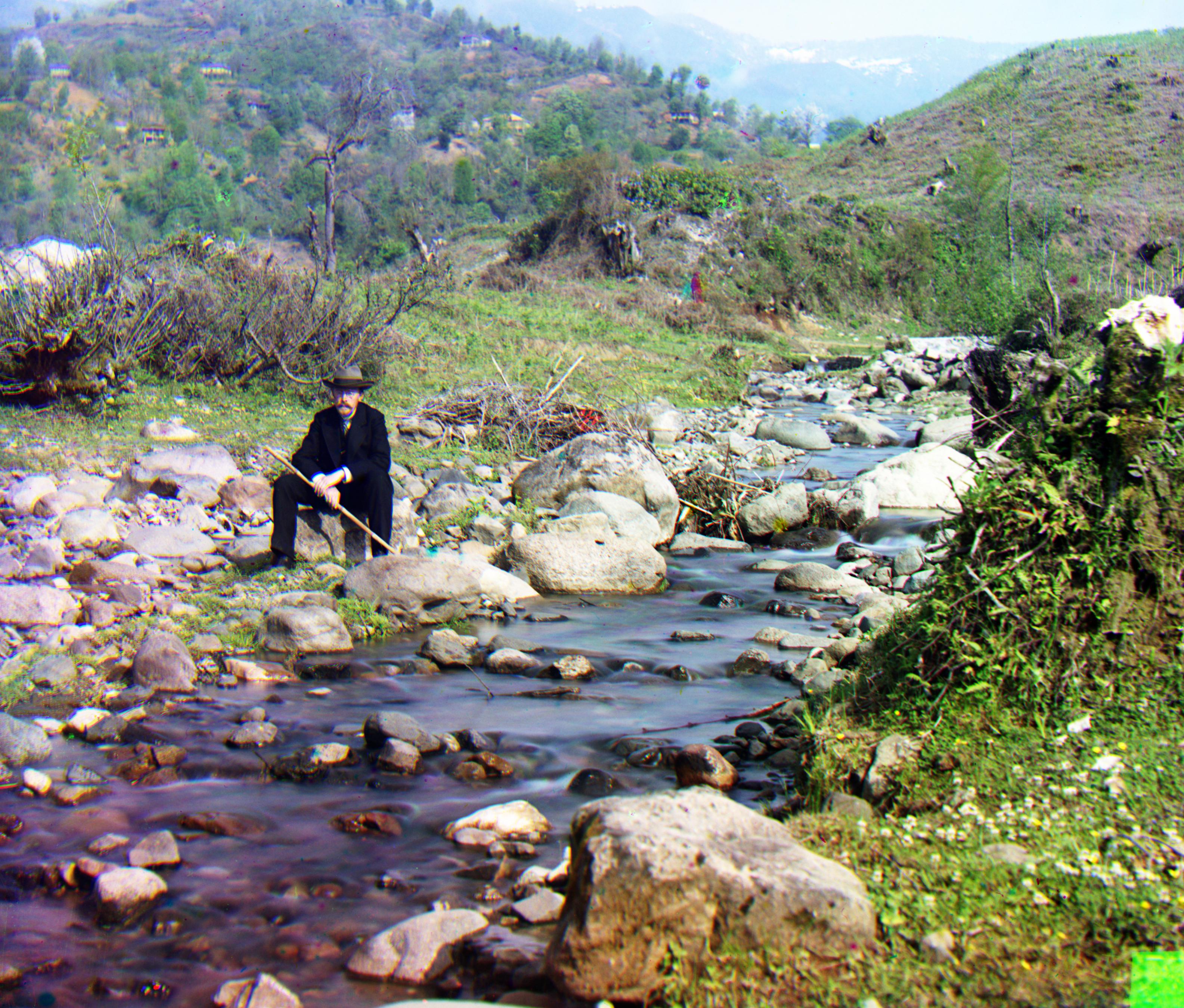
For the extra credit part of the project, I went ahead and used Histogram Equalization to make the images have a stronger contrast within the images so that they look much more appealing. This process essentially uses the intensities of the image found via the Histogram to make more uniform, thus weighing the intensities uniformally across the images. Two examples are shown below (hover over to see how they look after auto-contrasting was done). There are a few more examples displayed below at the "Bells and Whistles" image gallery below.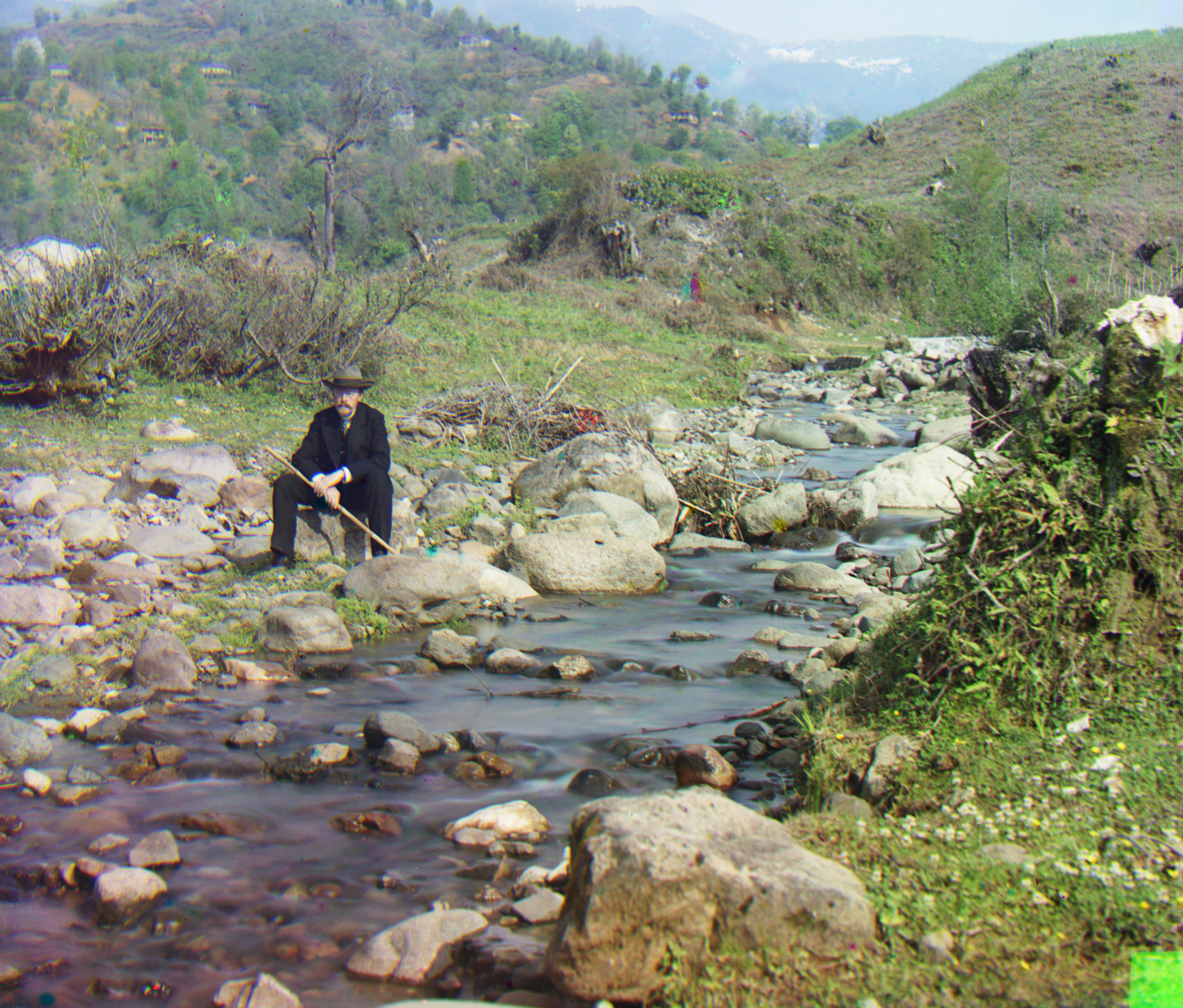
Results on example images:
Offsets are in the form of (Red X Offset, Red Y Offset) (Blue X Offset, Blue Y Offset)Cathedral: (7, 1) (-5, -2)
Runtime: 0.92s
Church: (35, -10) (-25, -5)
Runtime: 4.86s
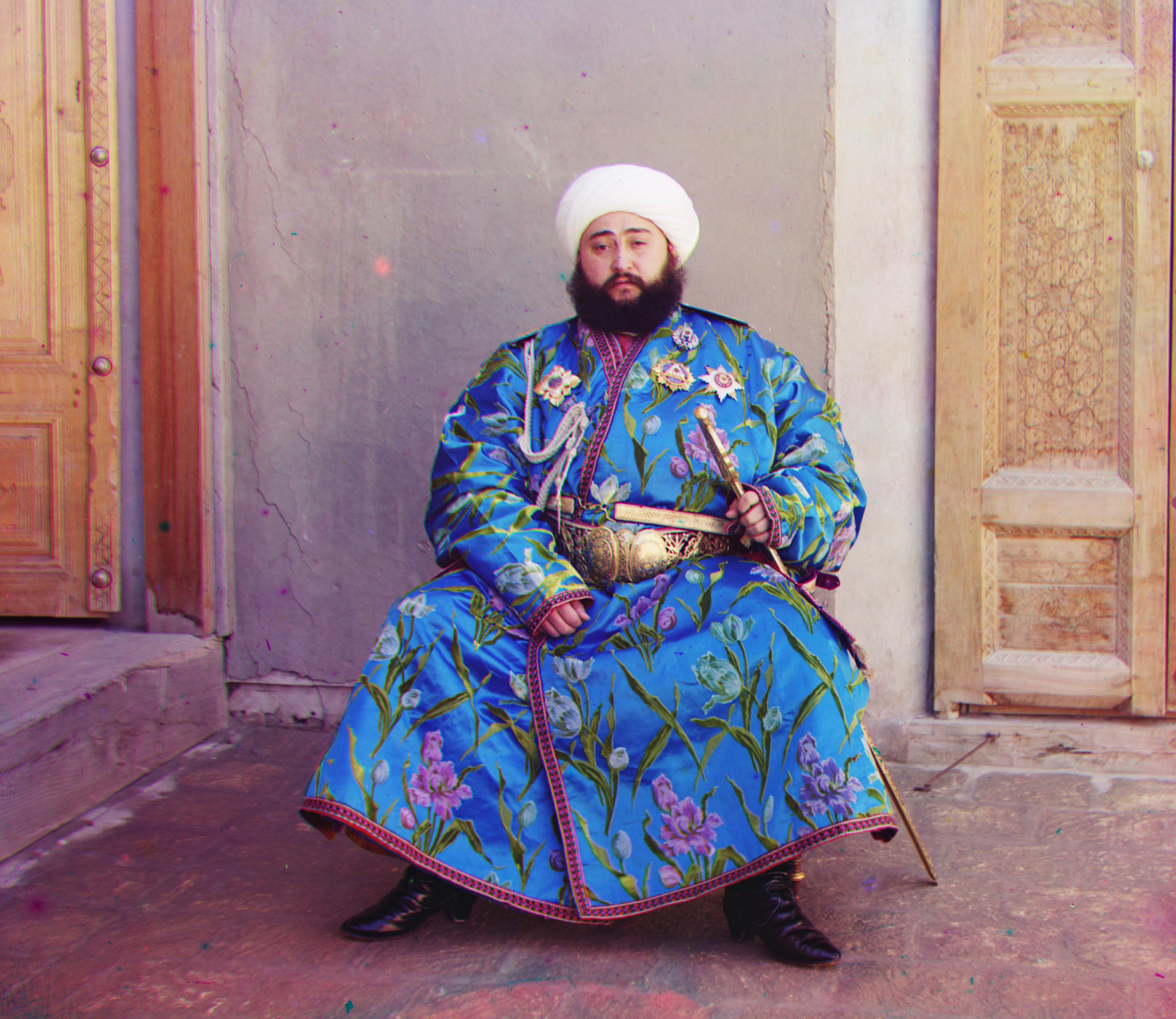
Emir: (55,15) (-50,-25)
Runtime: 3.21s
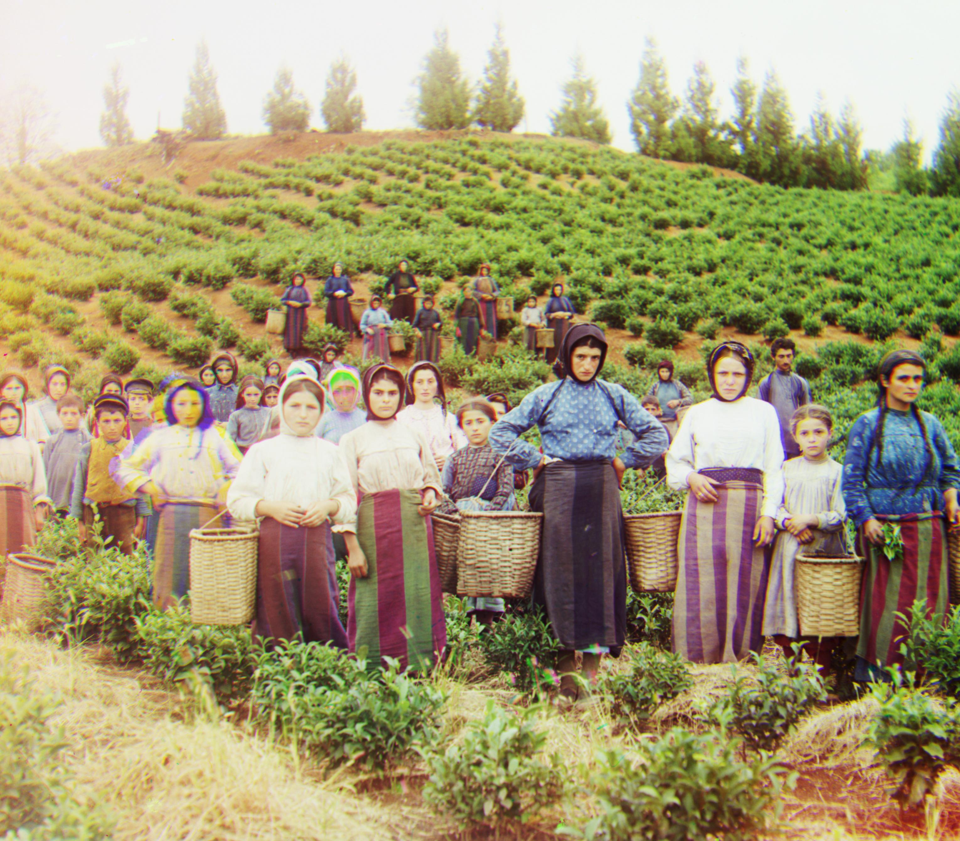
Harvesters: (65,-5) (-60,-15)
Runtime: 2.16s
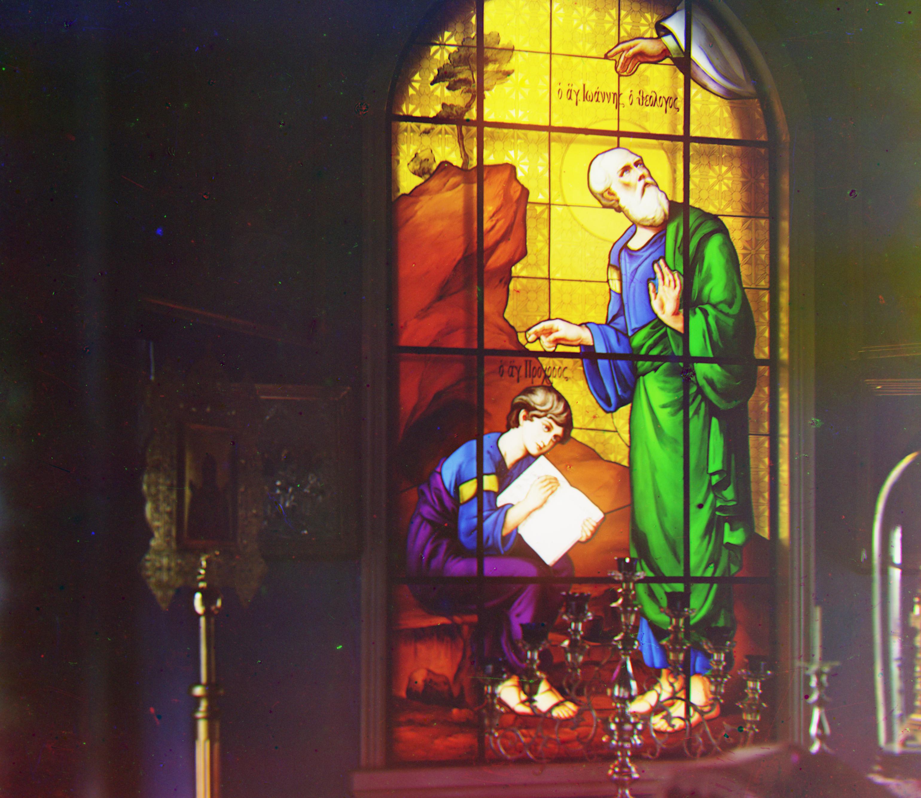
Icon: (50,5) (-40,-15)
Runtime: 3.68s
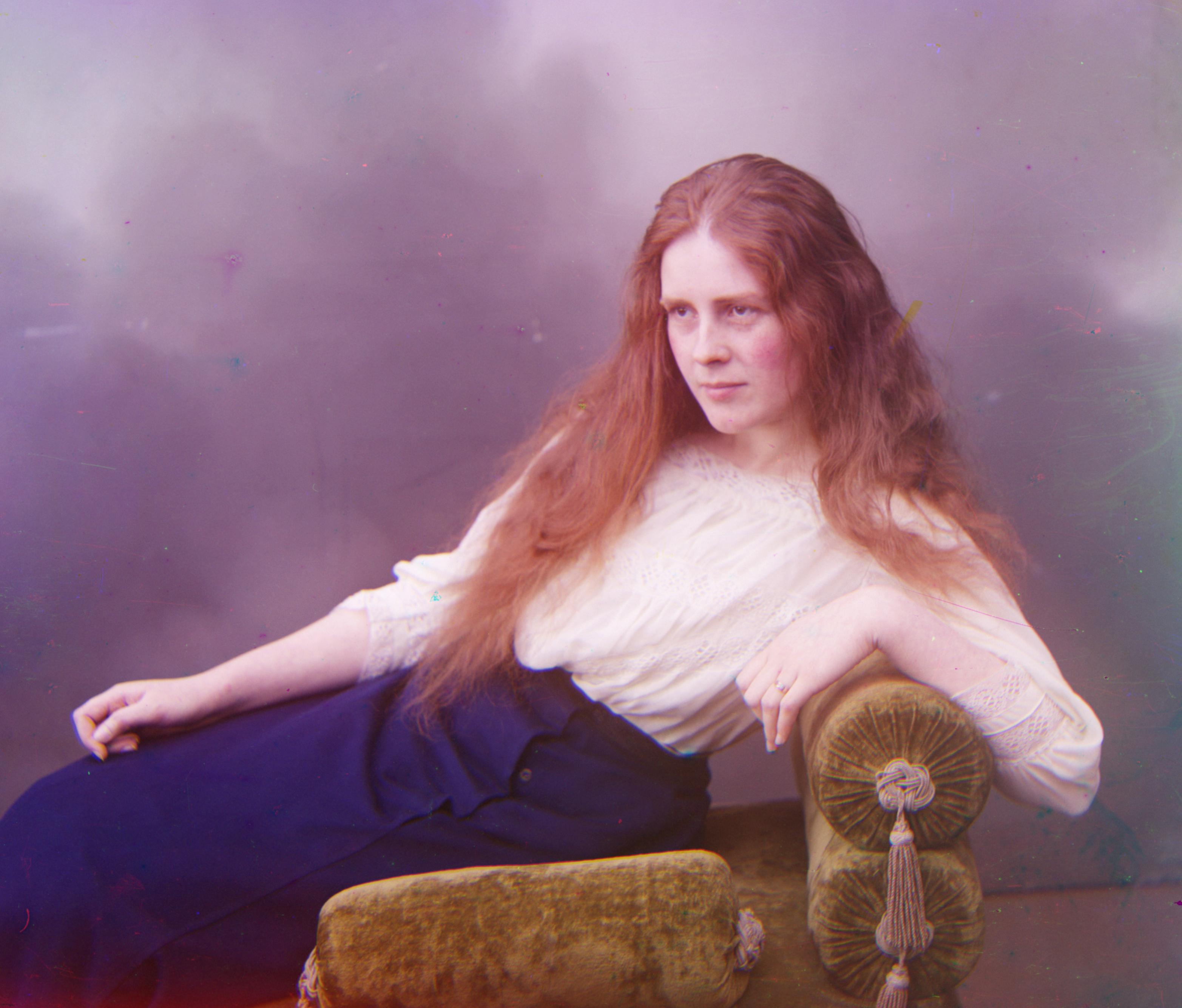
Lady: (60,5) (-50,-10)
Runtime: 3.39s
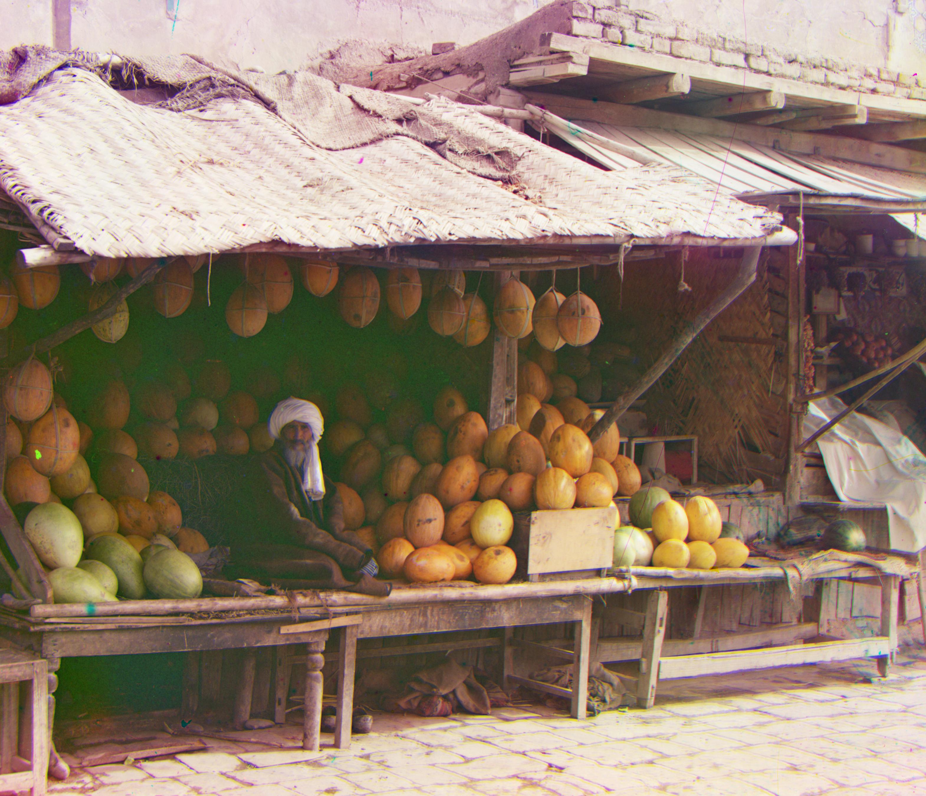
Melons: (95,5) (-80,-10)
Runtime: 3.32s
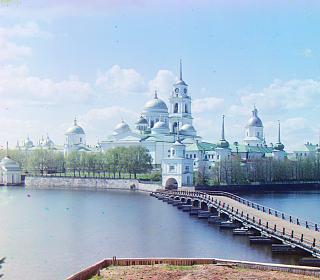
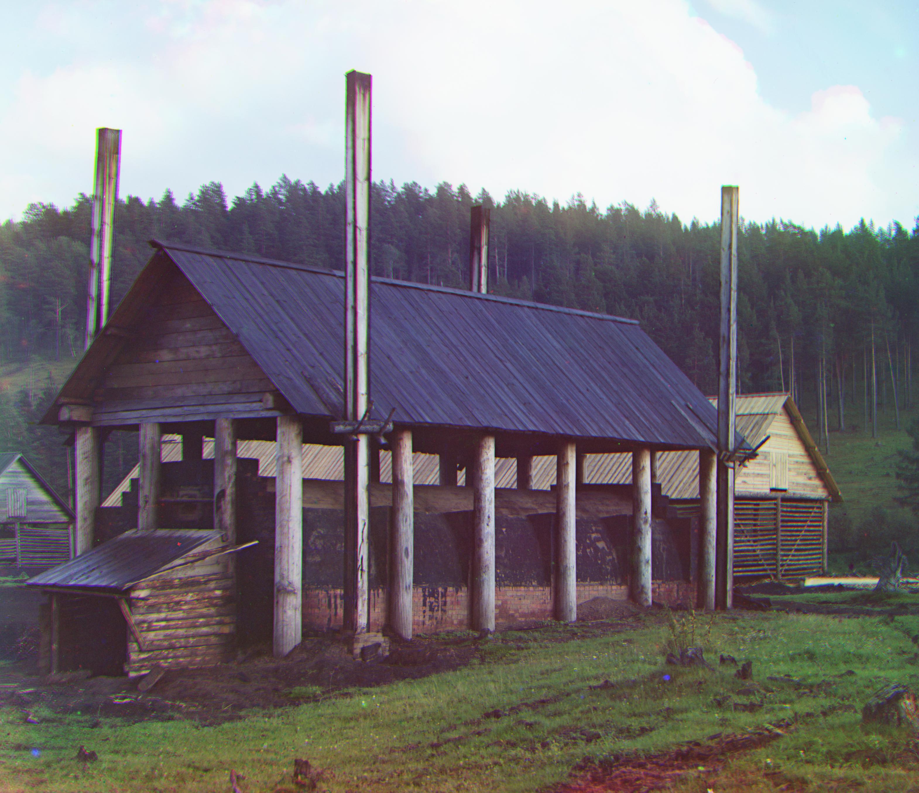
Monastery: (6,1) (3,-2)
Runtime: 1.25s
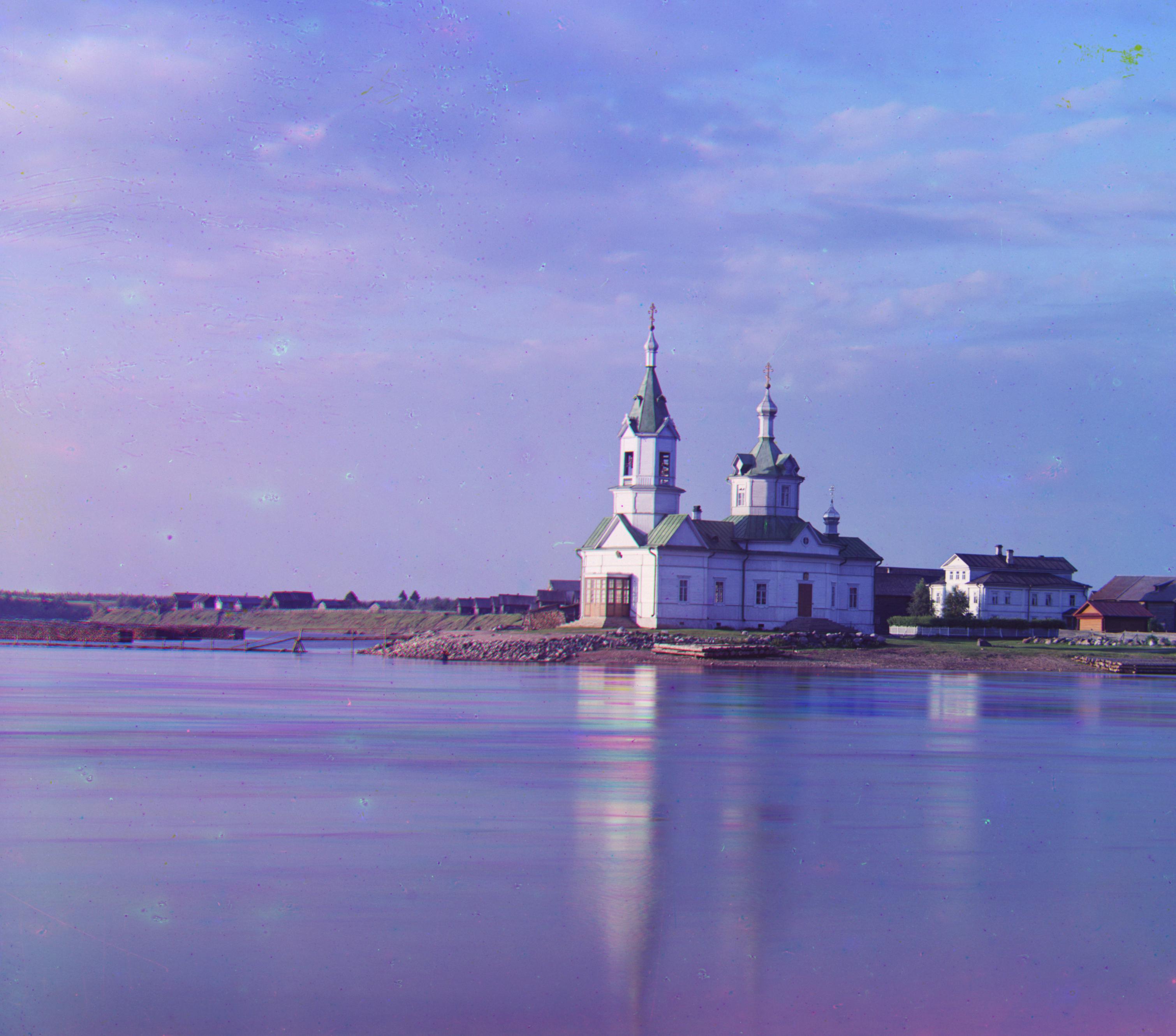
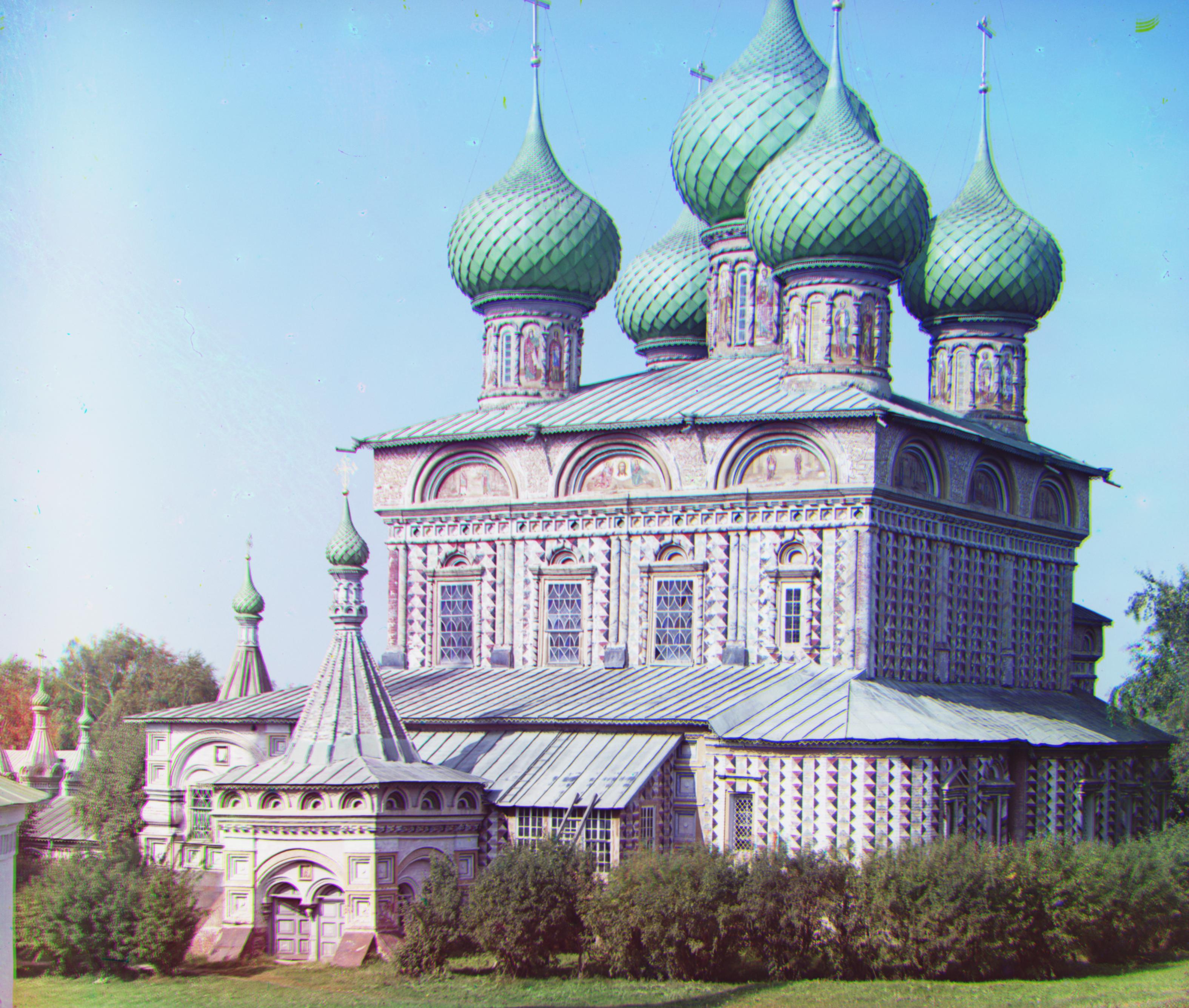
Onion Church: (55,10) (-50,-25)
Runtime: 3.34s
Self Portrait: (100,10) (-80,-30)
Runtime: 3.57s
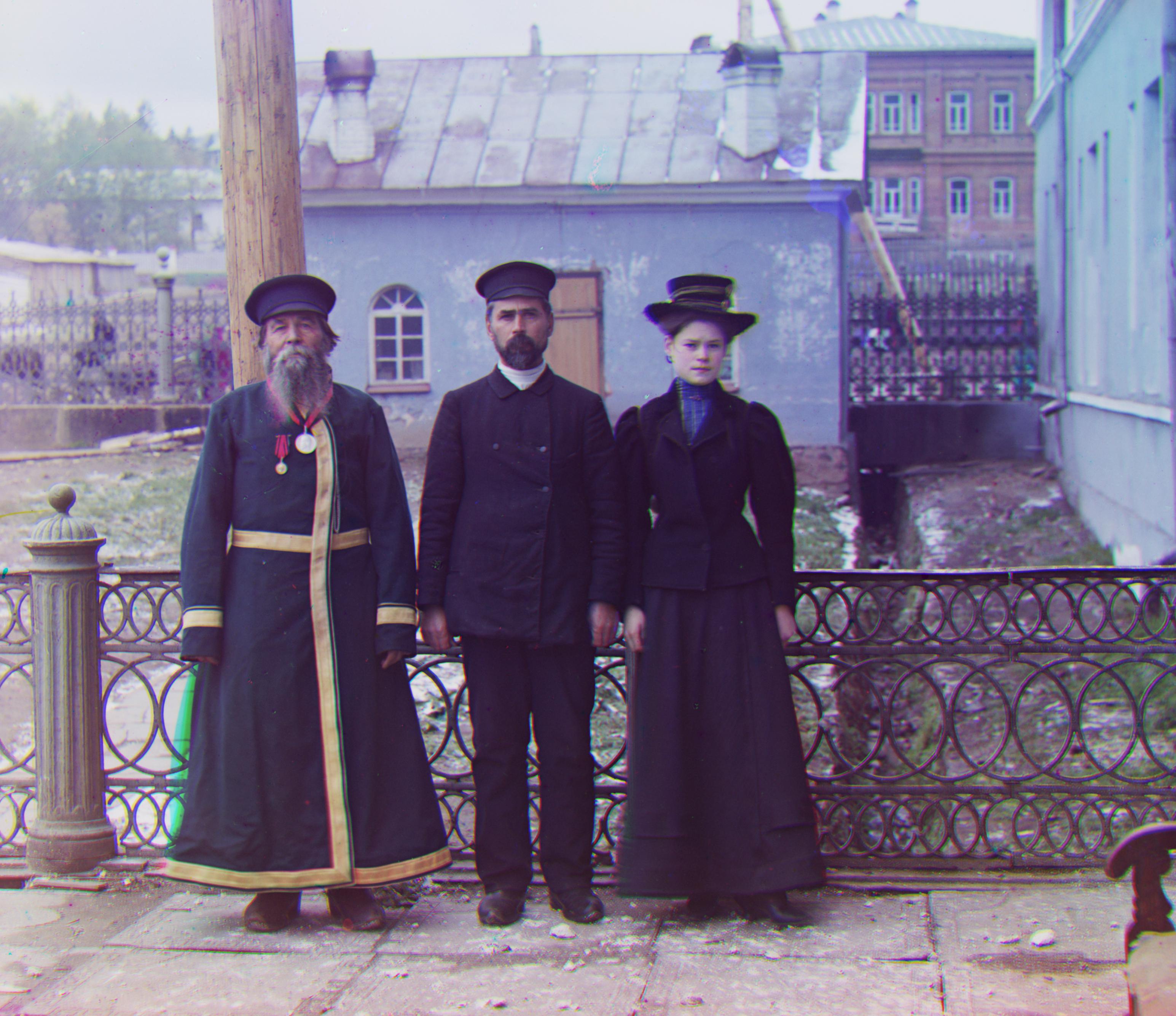
Three Generations: (60,0) (-50,-15)
Runtime: 3.14s
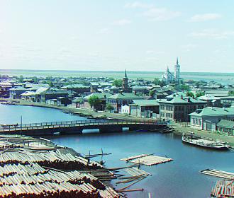
Tobolsk: (4,1) (-3,-3)
Runtime: 0.99s
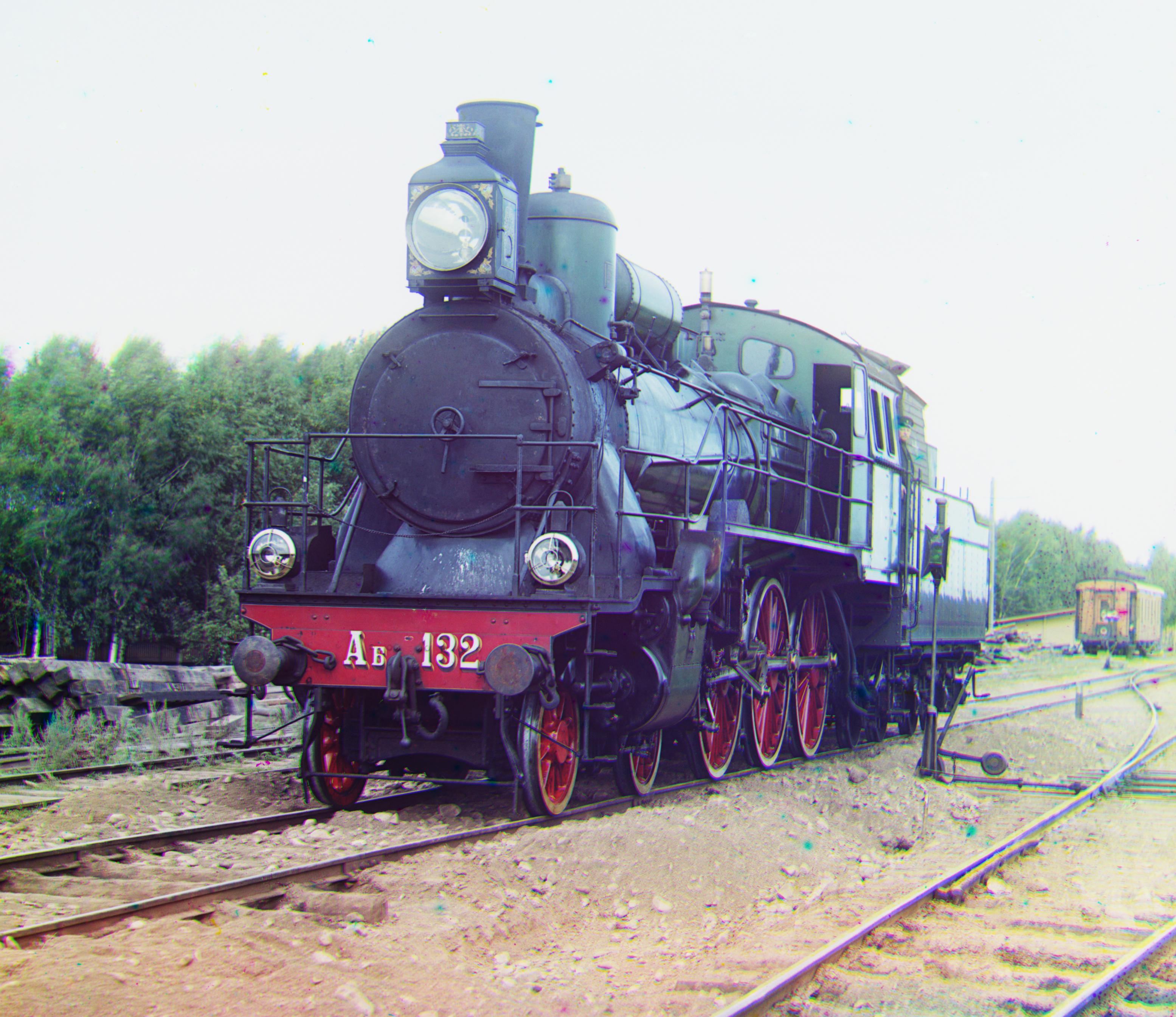
Train: (45,25) (-40,-5)
Runtime: 3.06s
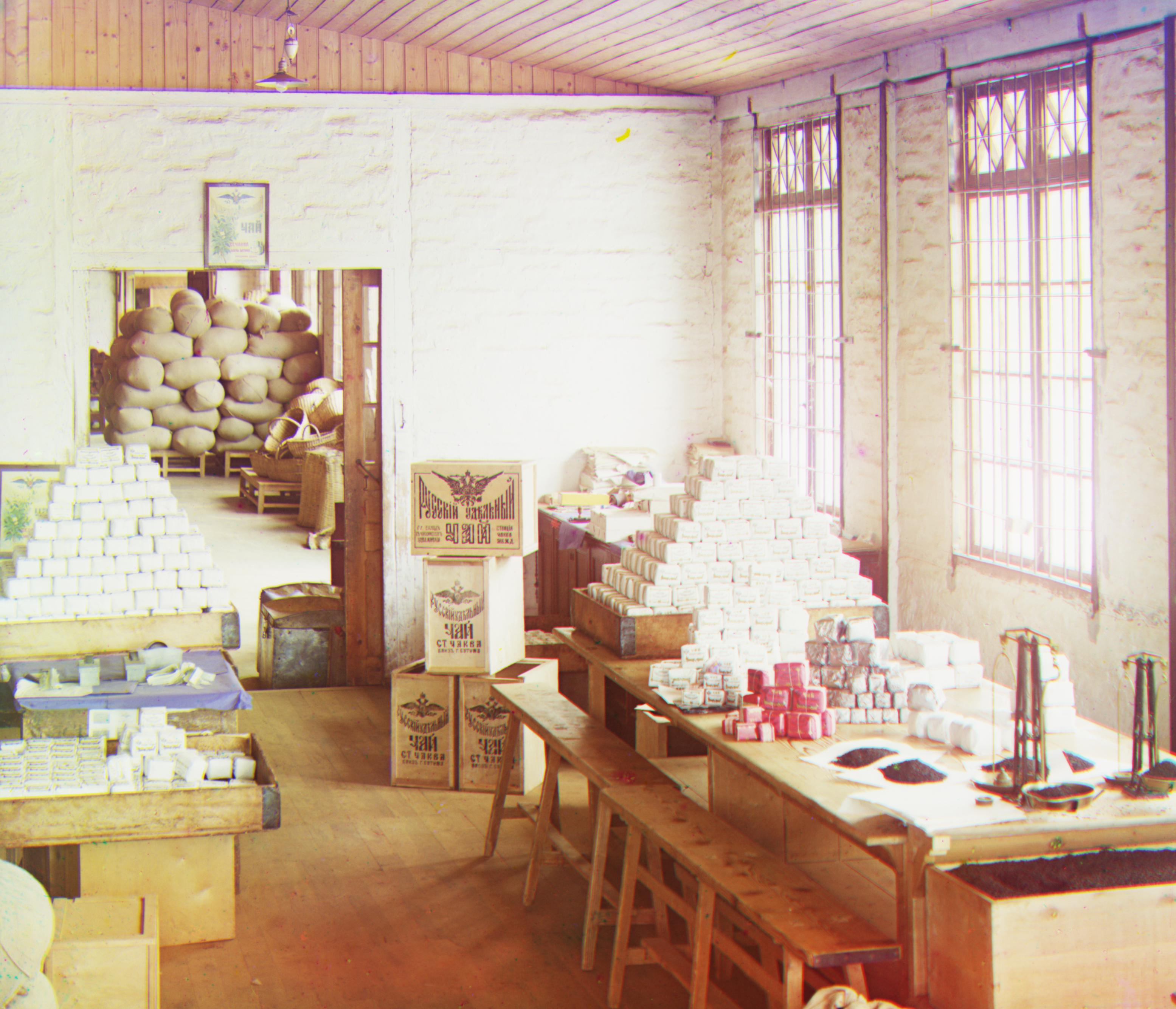
Workshop: (50,-10) (-55,0)
Runtime: 2.93s
Results on other images:
TIF/JPG Images taken from LOC
Bells and whistles
Easter Egg
Wow! You made it to the end of the webpage!
Lastly, an easter egg page here