Overview

Part I: Fun with Filters

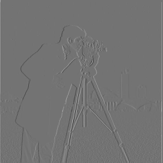
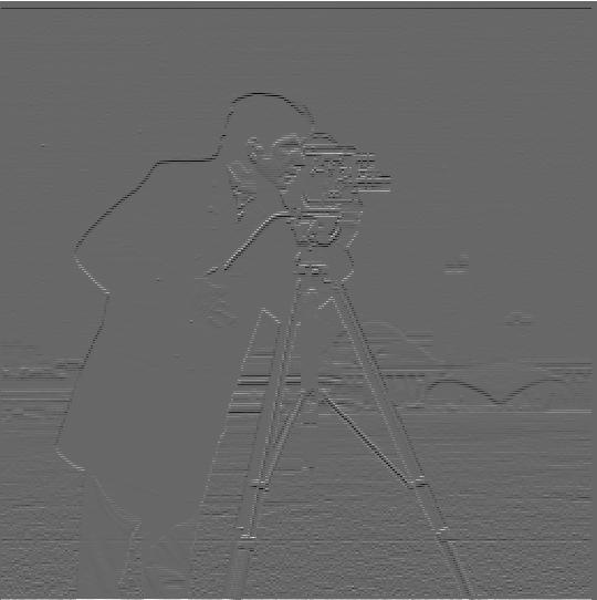
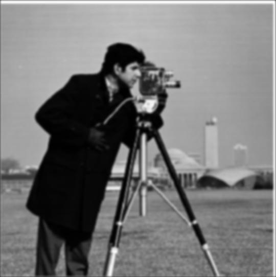
Part 1.1: Finite Difference Operator

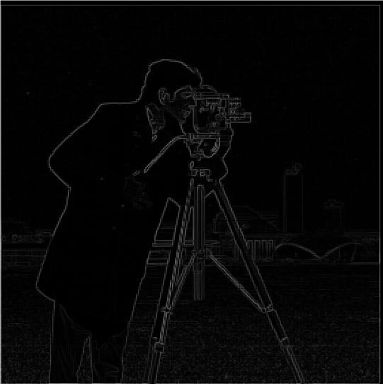
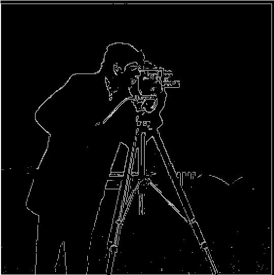
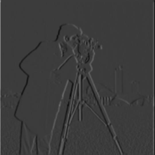
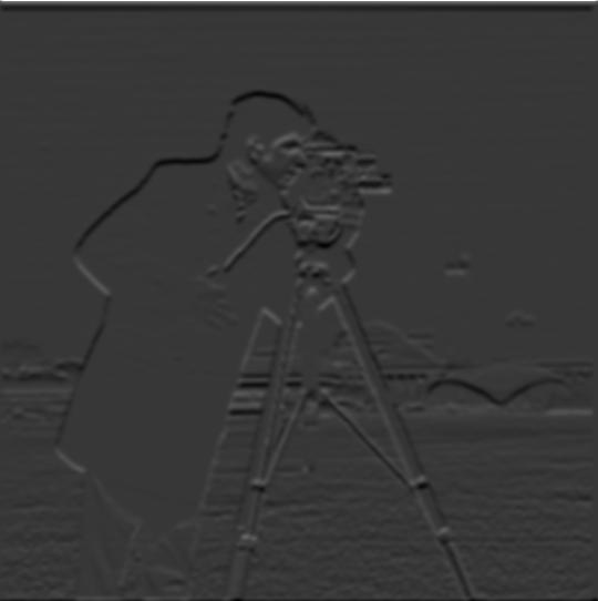
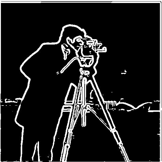
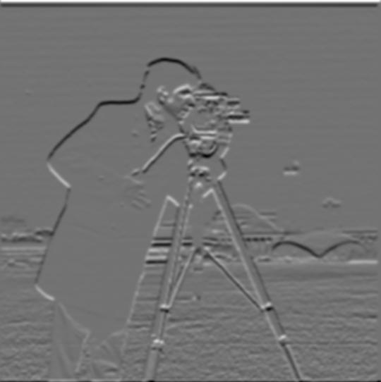
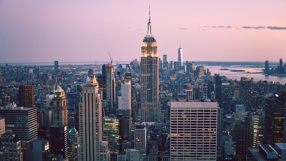
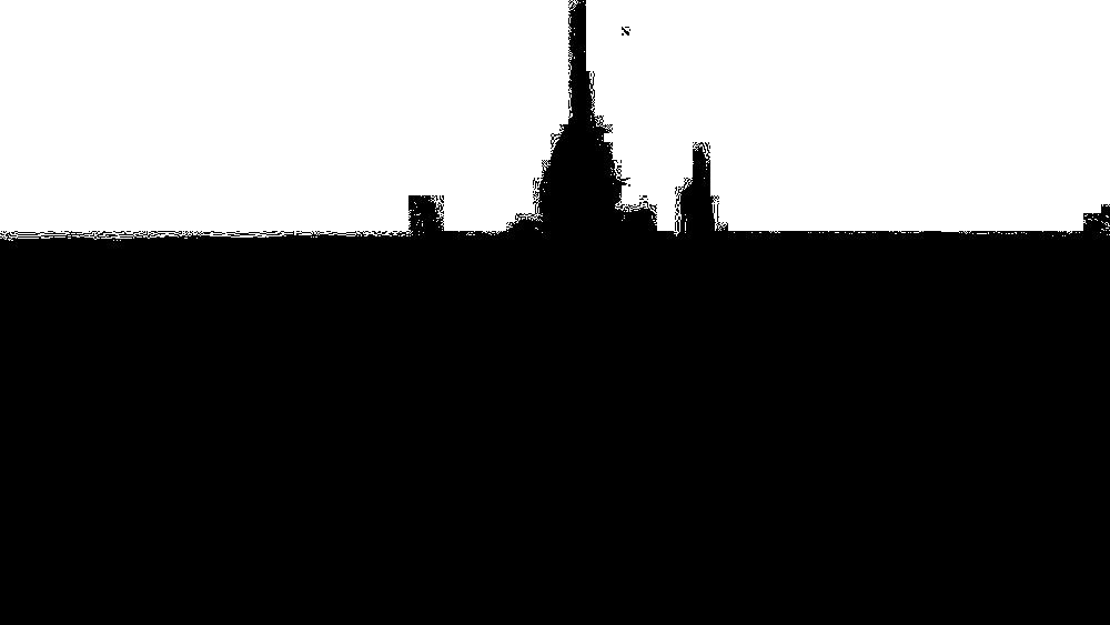
First, I convolved the provided image with the Dx and Dy operators respectively to retrieve the gradient elements wtih respect to x and y (ds/dx, ds/dy). To calculate the gradient magnitude image, I then element-wise squared each gradient subpart ((ds/dx, ds/dy)), sum them together, and took the square root to achieve the magnitude.

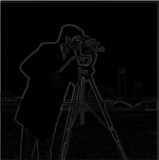
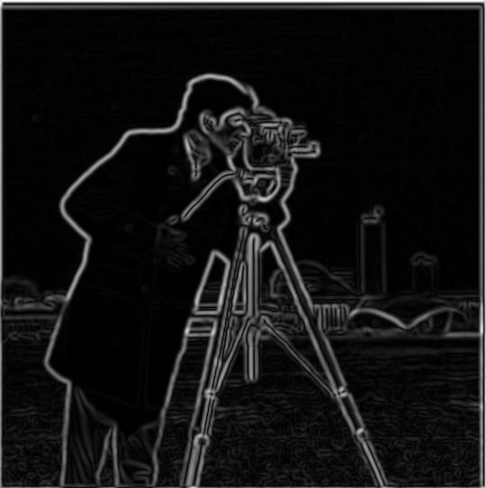
The edge image was computed by a binarization of the gradient magnitude with a threshold of 0.19. This means that every value above the threshold was set to 1 and set to 0 if below which helped remove the noise from the gradient image and resulted in the edges.

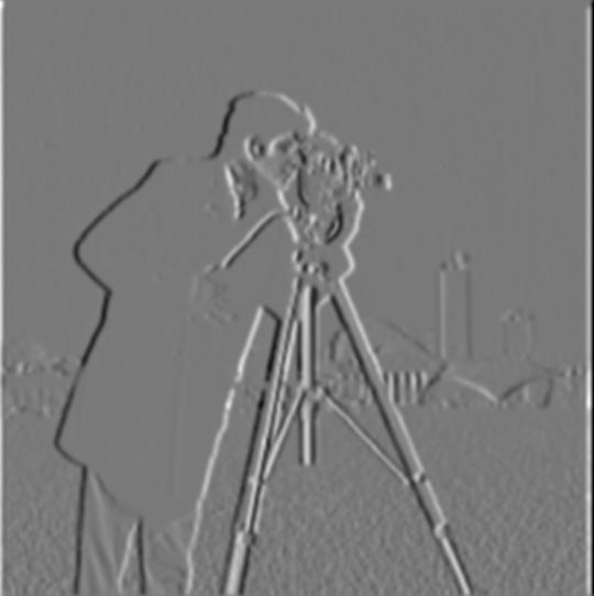
Part 1.2: Derivative of Gaussian (DoG) Filter

Gaussian Filter: ksize = 9, sd = 2

Edge Threshold: 0.04

Method 1: Blur image using Gaussian Filter, compute Dx Dy, find edge

The blurred image method provides a clearer edge image with significantly less noise compared to the edge image from Part 1.1. The edges in the blurred image are also thicker from the gaussian filter being a low pass filter.

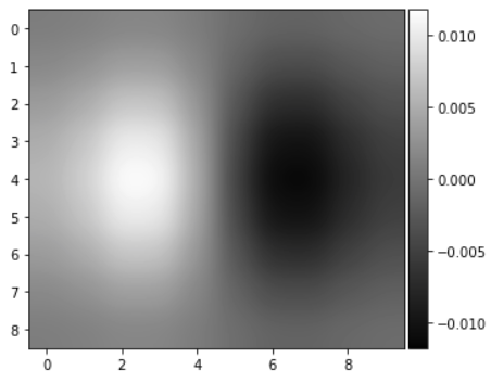
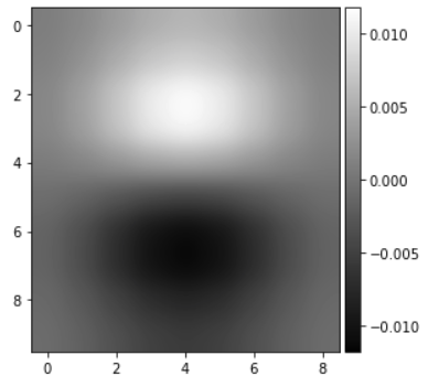
Method 2: Compute derivative of Gaussian filter, convolve with image, find edge

Alternatively, we can simply do 1 set of convolution with the image by first finding the derivatives of the Gaussian filter. As shown below, this yields the same results as the method described above.

Part 2: Fun with Frequencies!

Part 2.1: Image "Sharpening"

Using the unsharp masking technique, we can perform 1 convolution with a filter to artifically enhance the high frequencies by alpha. We can take our desired gaussian low-pass filter scaled by alpha and subtract it with 1 + alpha scale of the unit impulse filter. This newly created filter can be convolved with our image to amplify the high frequencies of the image, thus "sharpening" the image.

Sharpened Image = Sharpened Image * [(1 + alpha) Unit Impulse - alpha Gaussian Filter]

"taj.jpg", Gaussian Filter (ksize = 9, sd = 2)

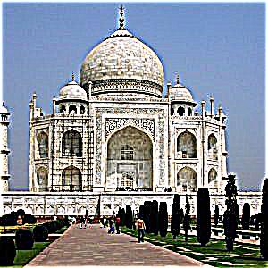
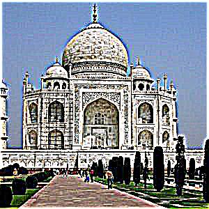
I also performed on extra examples depicted below. Some of these images, the high frequencies were overblowned to an unreasonable amount, see "nyc.jpg" alpha = 10 for an example.

Gaussian Filter (ksize = 9, sd = 2)

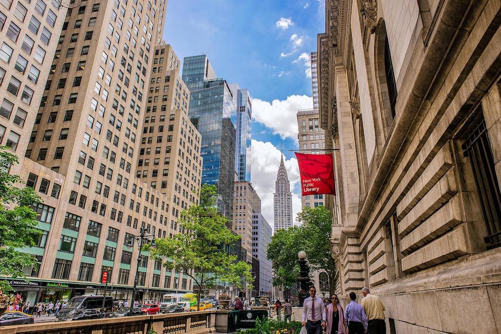
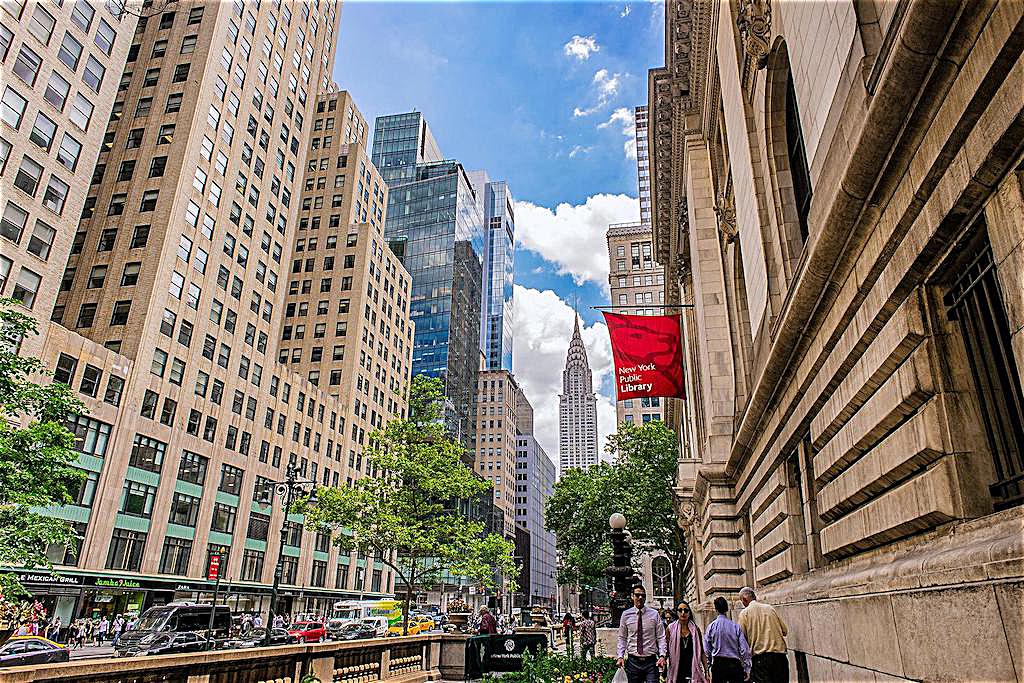
For experimentation, we can compare first blurring the image and then try to sharpen the image again. From the figures below, we can see that the resharpened image isn't exactly the same as the original image. This is because most of the high frequencies were lost in the blurring process.

Gaussian Filter (ksize = 30, sd = 5)

Part 2.2: Hybrid Images

We can create hybrid images by merging the low frequencies of one image with the high frequencies of another. The low frequencies are achieved convoluting the image with a Guassian filter and the high frequencies are achieved by creating a high pass filter through subtracting a gaussian filter with the unit impulse. Below are the results I achieved when merging.

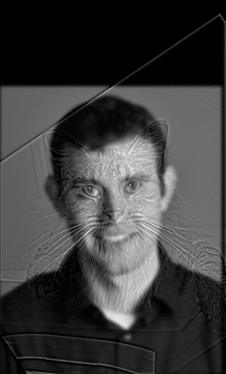
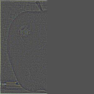
I also had some failures as shown when I try to merge two league of legends characters. Although we can easily see the ahri high frequencies, because of the lack of other features aligning the two images, we now essentially see an ahri cutout overlayed on a seraphine background. This is because the posture of each character in their respective images differ greatly thus the combined image results in something sub-optimal.

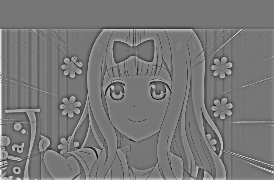
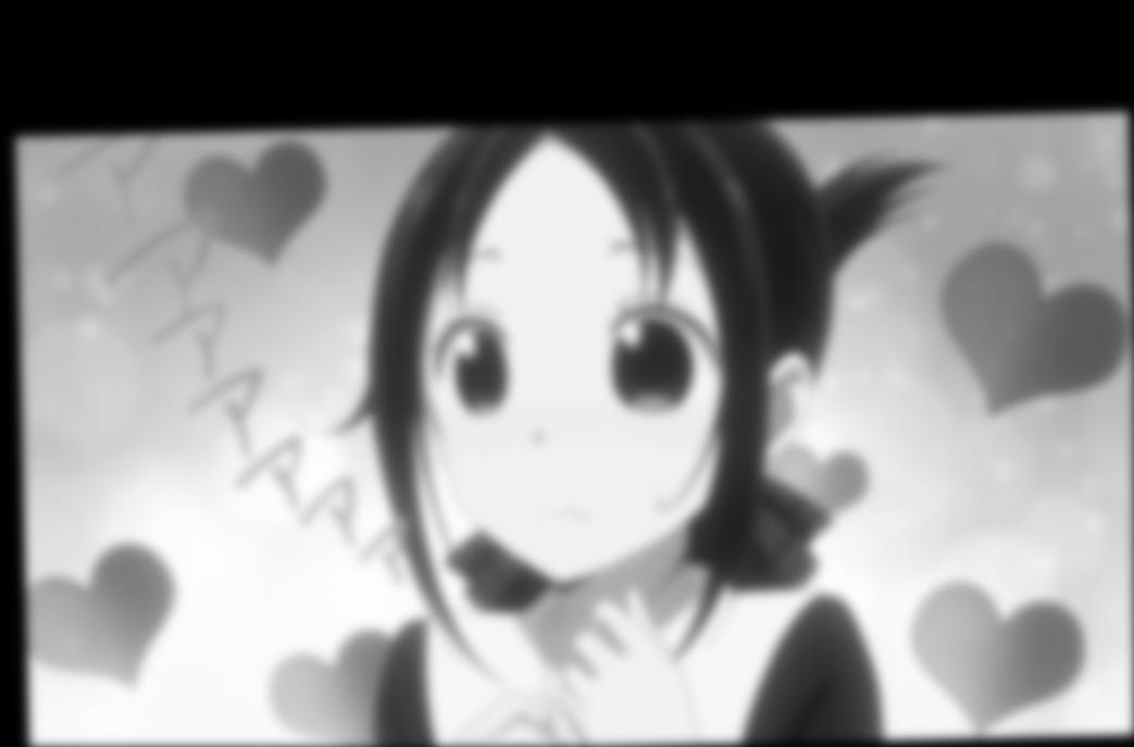
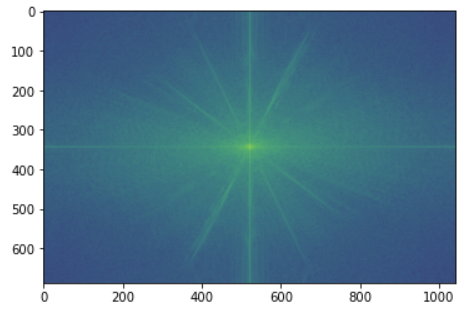
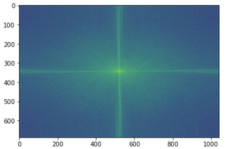
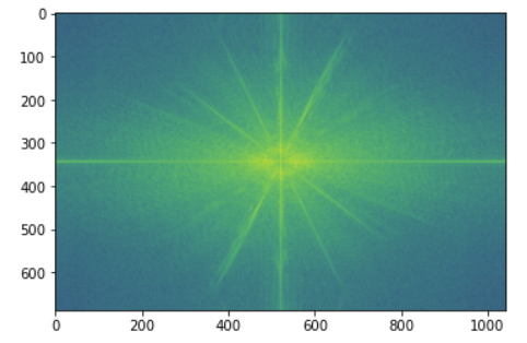
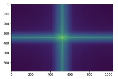
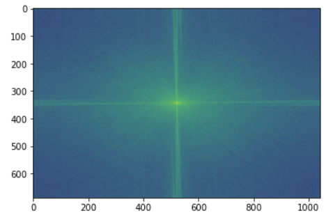
Here is the log magnitude of the Fourier transform of the two input images, the filtered images, and the hybrid image for kaguya and chika.

Part 2.3: Gaussian and Laplacian Stacks

For every image, we can create a Gaussian Stack and Laplacian Stack consistenting of fragments of the images. The Gaussian stack stores the blurred images as the image is passed thourgh various gaussian filters while maintaining the lower frequencies. The Laplacian stack is consisted of the mid band frequencies, computed by subtracting the ith Gaussian stack image by the (i+1)th Gaussian stack image - essentially the subtraction of 2 lower frequencies result in a mid band frequencies.

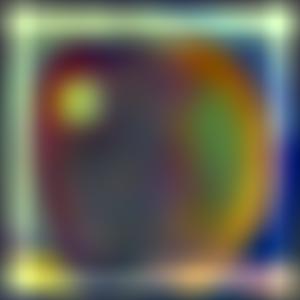
Using this, we can can utilize a mask to blend images together. By generating the laplacian stack of 2 images and generating the gaussian stack for a mask, we can blend the images as follows for each level.

LS = GR(LA) + (1 - GR) LB

where LS is the combined laplacian , GR is the gaussian for the mask region, LA is the laplacian of the image A, and LB is the laplacian of image B. In order to accommodate for the lack of a pyramid, for each subsequent Gaussian in the stack, we would double the ksize and sd to account for the missing downsampling from the stack.

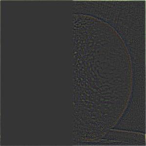
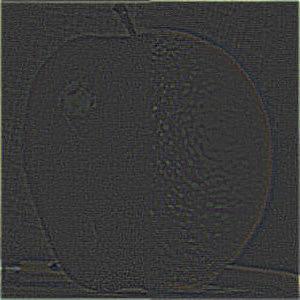
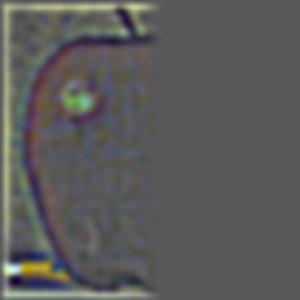
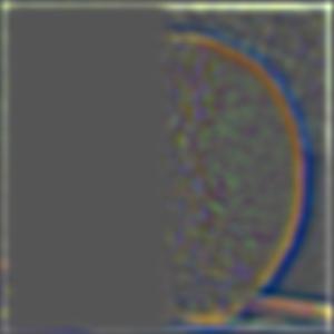
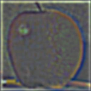
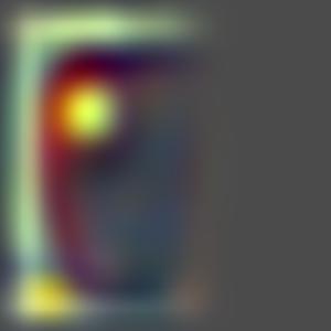
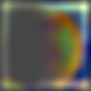
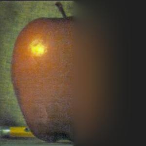
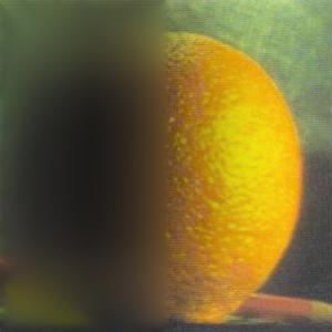
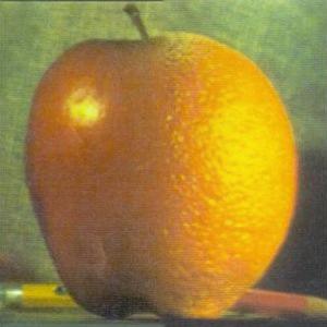
Below is an imitation of the Figure 3.42 from the Szelski book (page 167) through blending the laplacian matrices of the apple and orange together.

Gaussian Filter (ksize = 5, sd = 5) for initial blur (doubled each subsequent stack)

Part 2.4: Multiresolution Blending

To create a blend of two images, A and B, we only need to follow a few steps:

1. Create a binary mask consisting of only 0 and 1 indicating how you want to blend the image
2. Compute the mask's Gaussian stack
3. Compute both images' Laplacian stacks
4. Create a new combined Laplacian stack consisting of a blend of the two images' Laplacian stacks weighted by the Gaussian stack of the mask.

Here we have the orple constructed using a horizontal mask using an initial filter ksize = 5, sd = 5

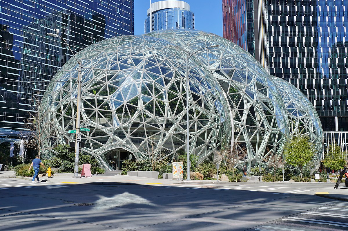
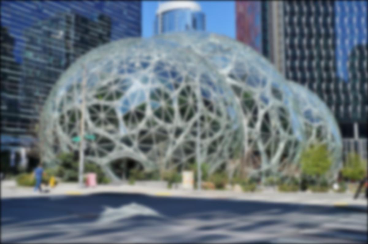
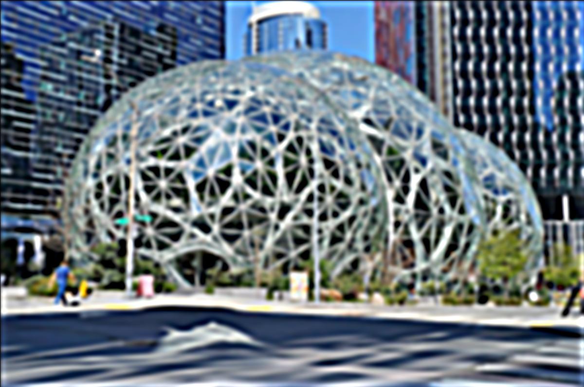
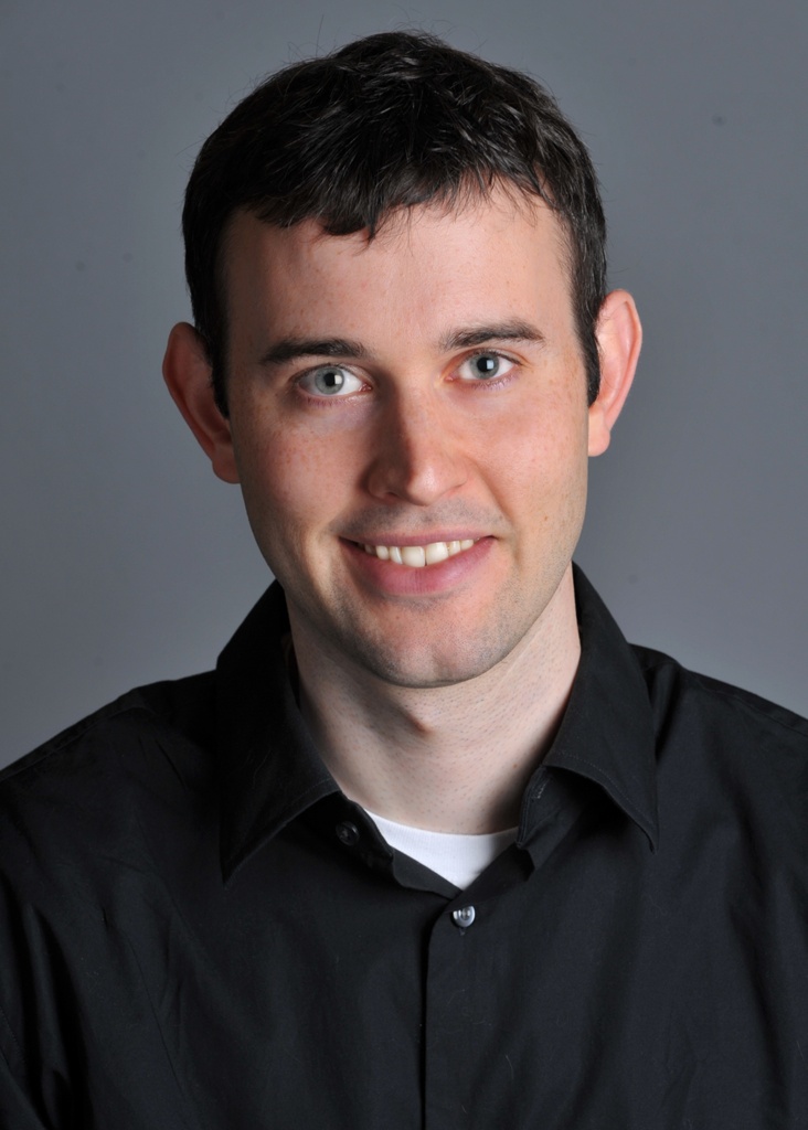
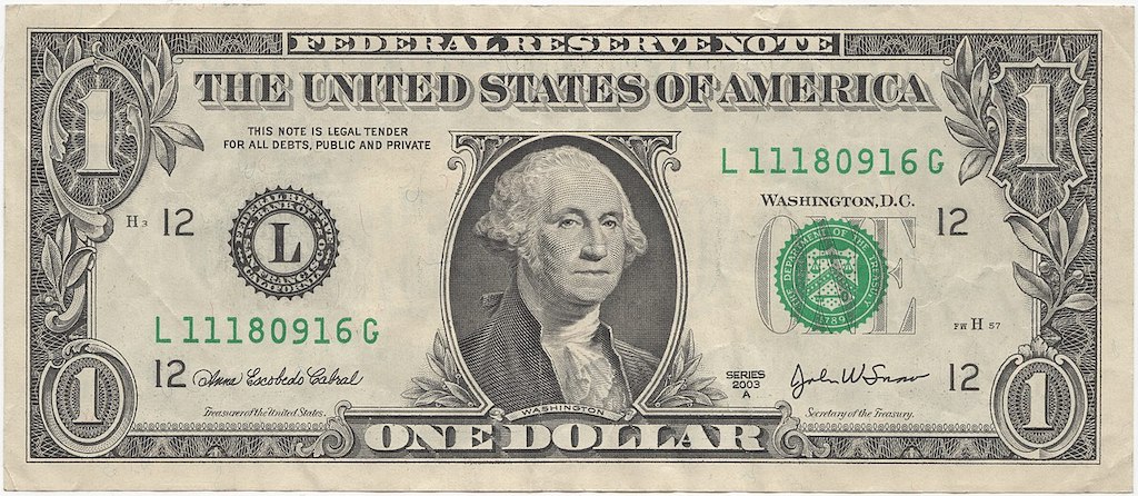
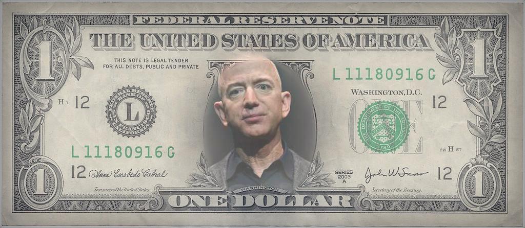
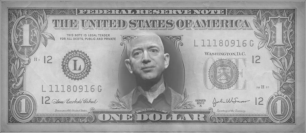
Now for some fun with custom images! (Using all 3 color channels!)

We have the dollar bill with George Washington as the face - an iconic symbol of the United States and we have the current richest man in the world - Jeff Bezos (founder of Amazon.com). Let's blend them together as the United States loves it's capitalism! Given the different color schemes of the pictures, grayscaling them makes it appear more realistic.

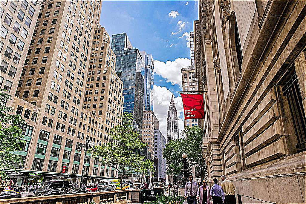
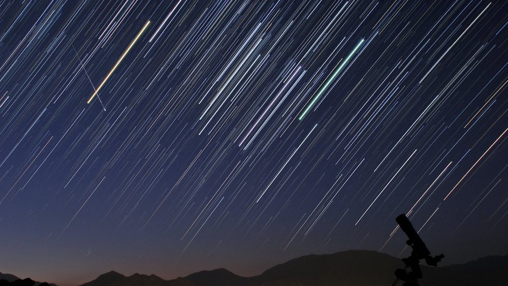
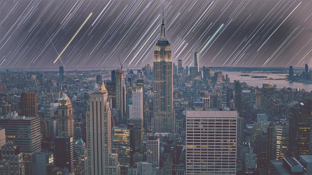
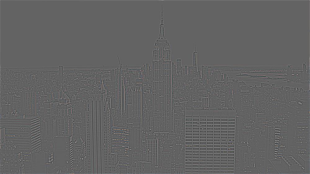
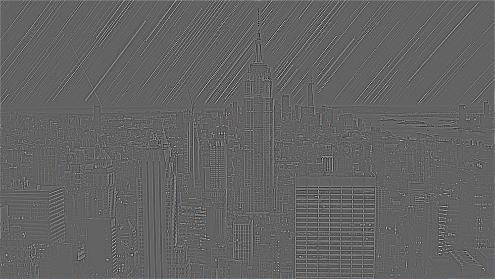
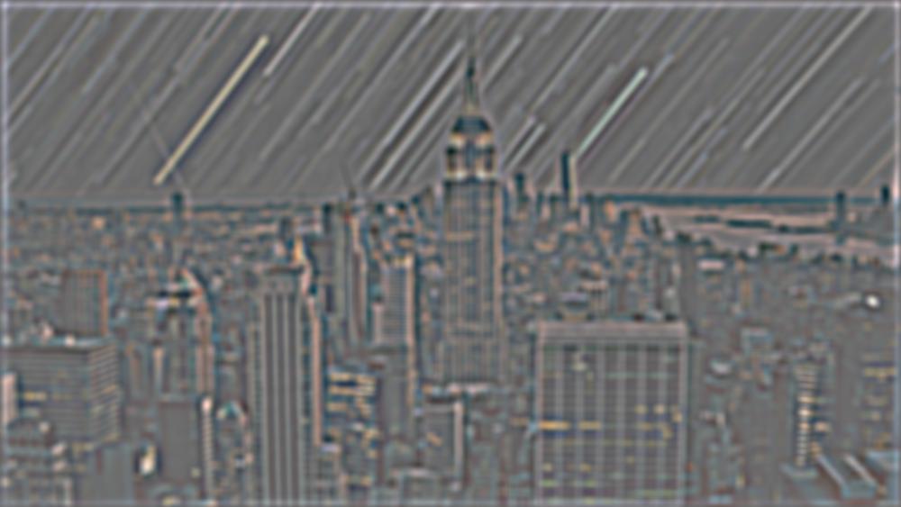
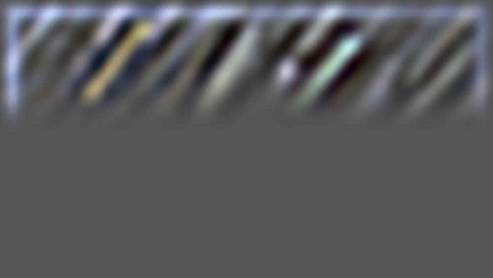
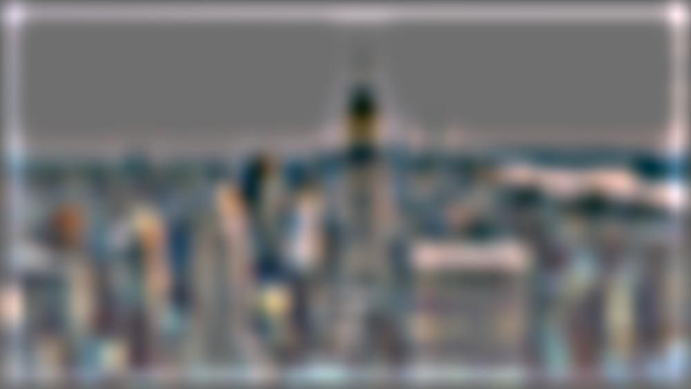
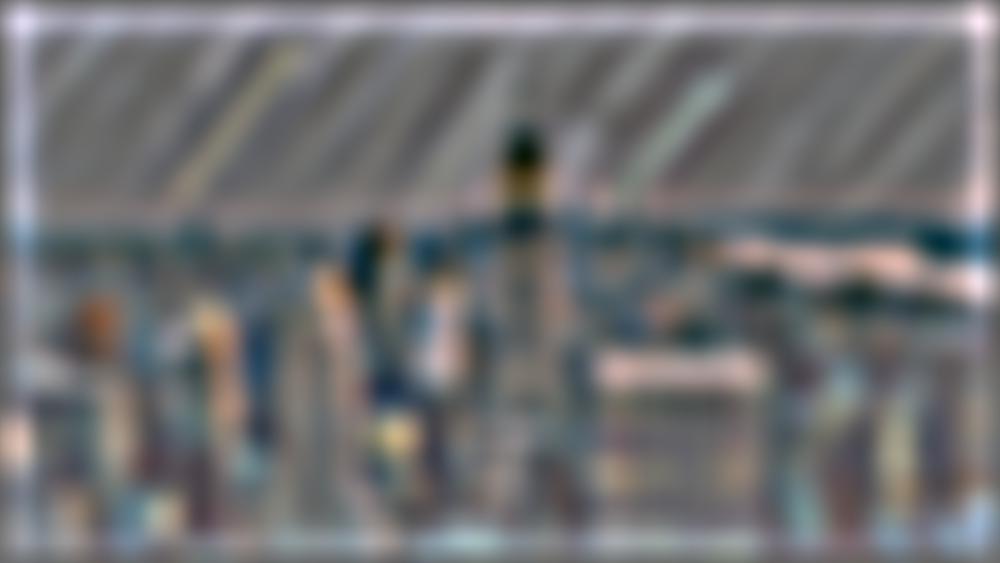
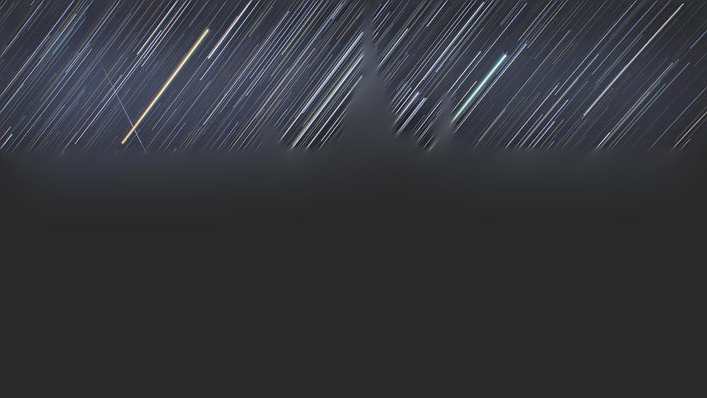
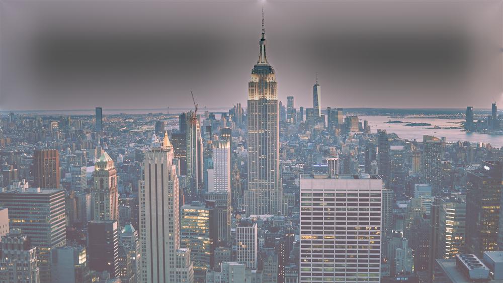
Inspired by the awesome visualizations of meteor showers, I decided to blend the NYC skyline with a meteor shower drawing just to see how it would turn out. Fortunately, it turned out wonderfully.

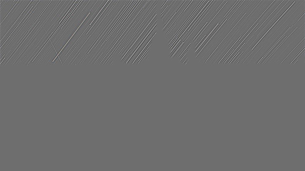
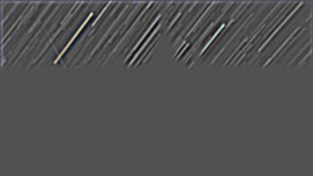
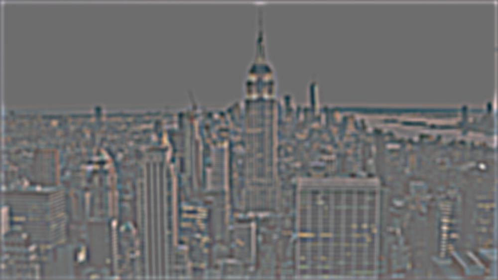
It actually looks very cool to see streaks in the night sky behind all the New York skyscrapers! Here is the Laplacian breakdown of the image.

Stack Size = 5, Initial Filter ksize = 5, sd = 5