Tony Lian’s Project 2

· (15 points) Include a brief description of gradient magnitude computation.

· (15 points) Answer the questions asked in part 1.2

Part 1: Fun with Filters

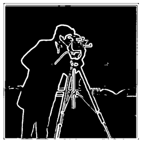
Part 1.1: Finite Difference Operator

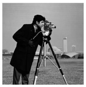
Original Image:

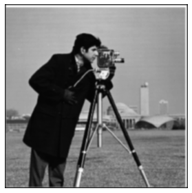
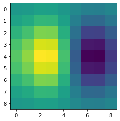
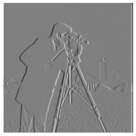
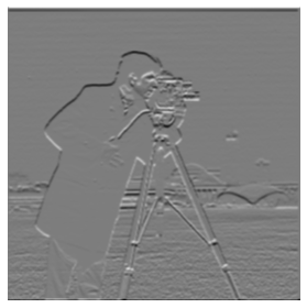
Partial derivatives (w.r.t x and y):

This is computed with a convolution to a derivative filter.

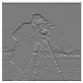
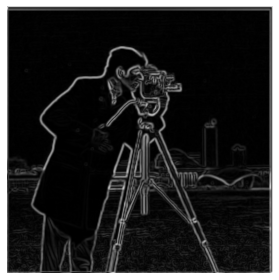
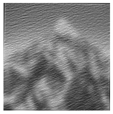
Gradient magnitude image:

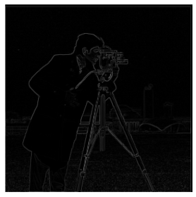
This is computed with (grad_x ** 2 + grad_y ** 2) ** (0.5) in Python syntax, which is taking the norm of a vector with grad_x and grad_y of each point.

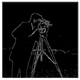
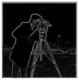
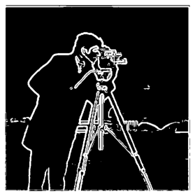
Binarized gradient magnitude image (threshold: 0.2):

Part 1.2: Derivative of Gaussian (DoG) Filter

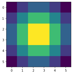
Gaussian kernel with sigma=2, width=6:

Blurred image (with a Gaussian kernel, sigma=2):

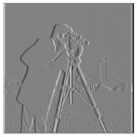
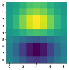
Partial derivatives (w.r.t. x and y):

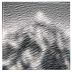
Gradient magnitude:

Gradient magnitude (binarized):

· What differences do you see?

It’s much clearer with much less noise, especially on the grassland with more distrations.

To fuse two filters, we can create the convolution of them with

G_x = scipy.signal.convolve2d(gaussian_kernel_2d, D_x, mode="same", boundary="fill")

G_y = scipy.signal.convolve2d(gaussian_kernel_2d, D_y, mode="same", boundary="fill")

The derivative of gaussian filter (x and y):

· Verify that you get the same result as before.

Partial derivative with gaussian in one filter:

Magnitude and the binarized one:

It looks the same as the one with two separate filters.

Part 2: Fun with Frequencies!

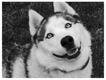
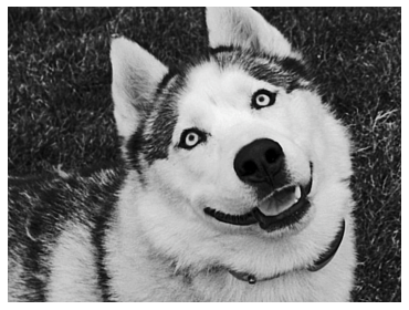
Part 2.1: Image "Sharpening"

Sharpening comparisons (left: origin, right: sharpened):

The edges are clearer on the right.

Filter merging formula (from the slides in lecture):

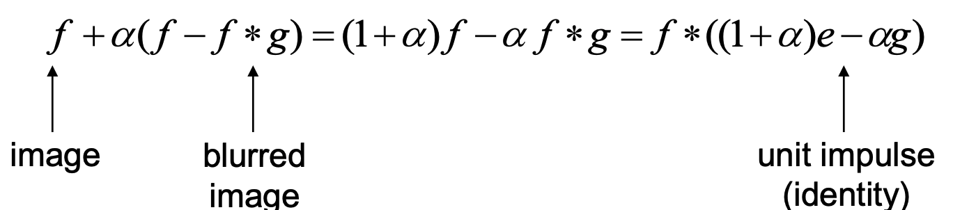
Implementation of merging filter:

merged_kernel = -alpha * gaussian_kernel_2d.copy()

merged_kernel[

gaussian_kernel_2d.shape[0] // 2, gaussian_kernel_2d.shape[1] // 2] += alpha + 1

Merged kernel leads to the same output:

My image (left: original, right: sharpened):

The texture on the back is more visible.

My image -> blurred -> sharpened:

Look at the lower right, sharpened image recovers some texture from the blurred image.

Part 2.2: Hybrid Images

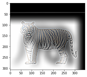
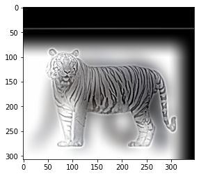
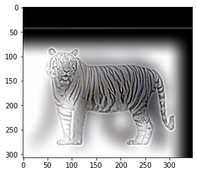
My favorite image (a tiger and an elephant):

Fourier transform with their original images:

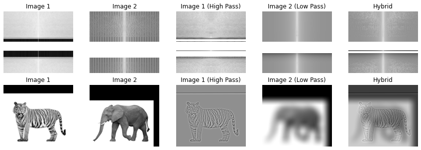
The high pass filter removes the part with low frequency, and the low pass filter removes the information with high frequency.

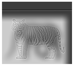
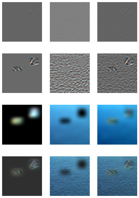
Cat with two positions:

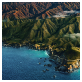
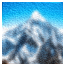
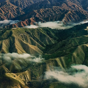
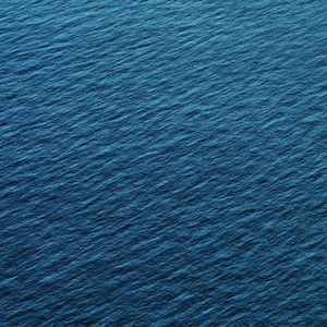
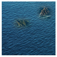
Mountain and sea (can be seen as a failure case – sea could not be recognized clearly):

Bells & Whistles (Extra Points)

Colored hybrid images (Color foreground vs Color background vs Color both):

For these two images, coloring background makes the foreground less visible, and coloring foreground gives a sense of the sea.

Color foreground vs Color background vs Color both:

Note that coloring foreground makes it more visible. Coloring background makes less sense, possibly because we are less good at sensing subtle color variation at background (with most of the cells rods, which do not perceive color).

Therefore, coloring foreground is the best for hybrid images.

Multi-resolution Blending and the Oraple journey

Part 2.3: Gaussian and Laplacian Stacks

Visualizations of Gaussian and Laplacian Stack

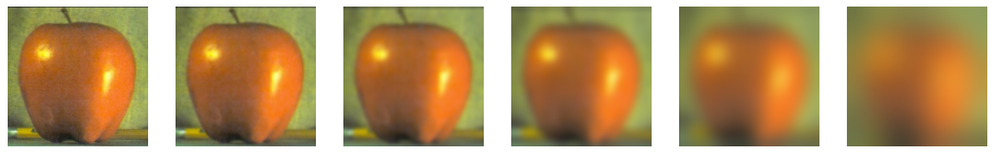
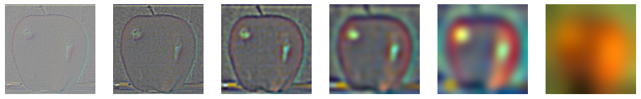
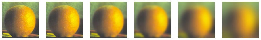
Blending levels of the stack

Blend

Part 2.4: Multiresolution Blending (a.k.a. the oraple!)

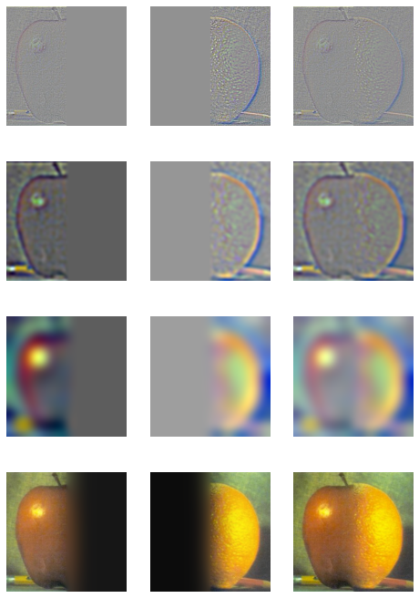
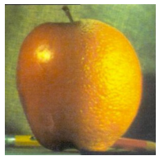
The apple with orange (as in Part 2.3):

My favorite one:

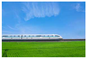
Two images:

Mask:

Blend:

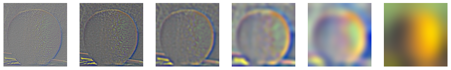
Laplacian stack grain to coarse from top to the bottom:

Another pair:

Image1:

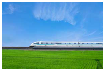
Image2:

Mask:

Blend:

Laplacian stack:

Bells & Whistles (Extra Points)

· Try using color to enhance the effect. (2 points)

I’ve been using the colored version throughout the assignment.

Additional note: since the merging process is fully linear (convolution with a Gaussian filter is linear) and applies the same way to all channels, to get greyscale blended image as if the inputs are greyscale, just turn them into greyscale by multiplying with conversion matrix (i.e. converting the inputs to greyscale is the same as converting output to greyscale) because matrix multiplication is linear.

Tell us what is the coolest/most interesting thing you learned from this assignment!

I learned how to make these amazing images.