CS 194-26 Project 2 Report

Part 1: Fun with Filters

Part 1.1: Finite Difference Operator

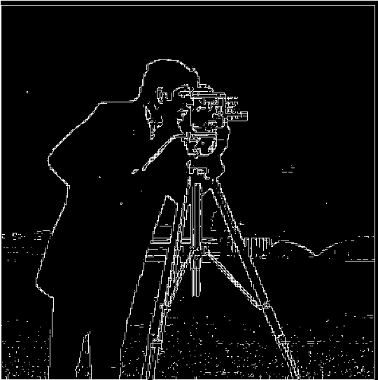
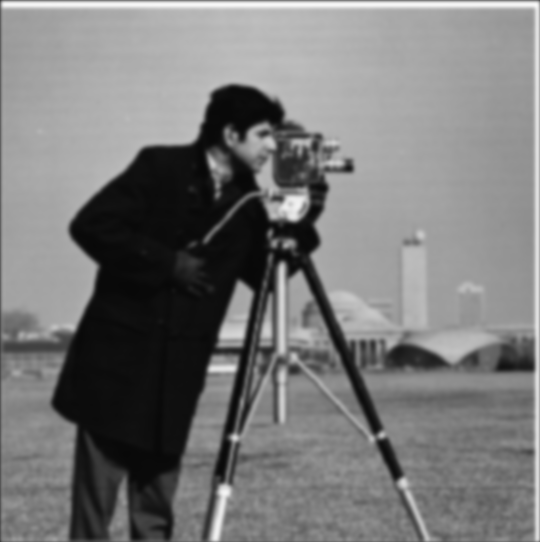
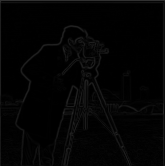
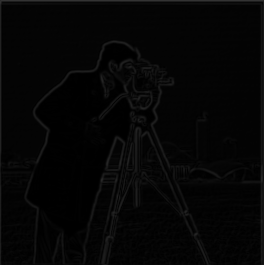
In this part of the project, I will convolve the cameraman image with finite difference operators in order to obtain a gradient magnitude image for the cameraman image. From the obtained gradient magnitude image, I create another image where the edges of the gradient magnitude image are sharpened. Here is the original cameraman image:

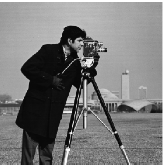
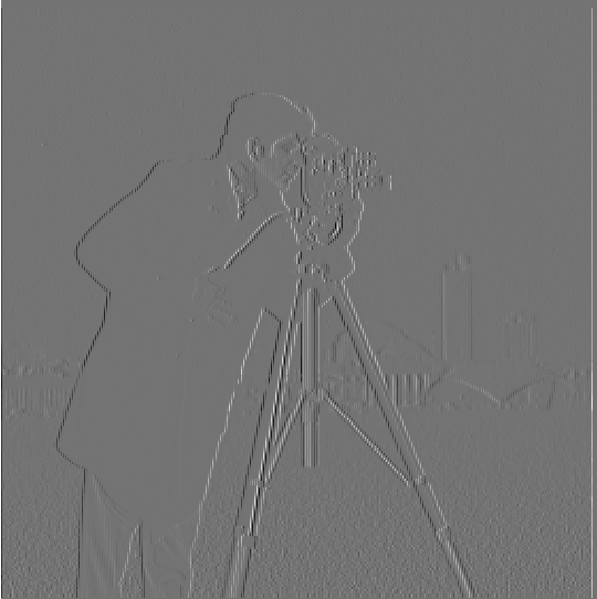
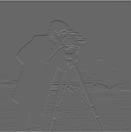
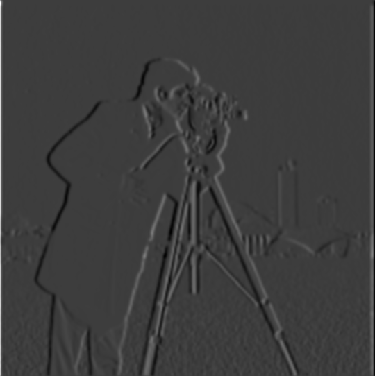
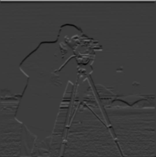
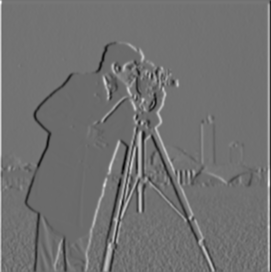
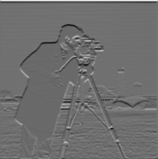
We have the following two finite difference operators: \(D_x=\begin{bmatrix} 1 -1 \\ \end{bmatrix}\), \(D_y=\begin{bmatrix} 1 \\ -1 \\ \end{bmatrix}\). I use scipy.signal's convolve2d function to convolve \(D_x\) and \(D_y\) around respective copies of the cameraman image. 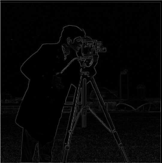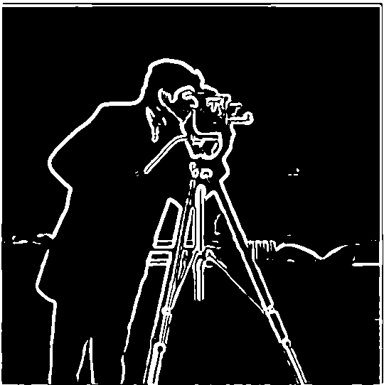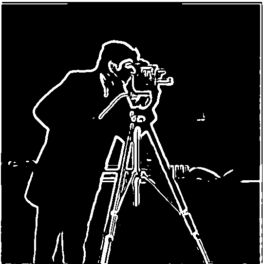After obtaining the two resulting images (one from convolving the cameraman image with \(D_x\) and the other from convolving the cameraman image with \(D_y\)), I compute the gradient magnitude image by taking the square root of the squares of the two convolvements, displayed in equation \[\sqrt{(D_x * \text{cameraman})^2 + (D_y * \text{cameraman})^2}\] where the operations are applied pixel-wise to produce the final gradient magnitude image. From there, I try to highlight the edges of the gradient magnitude image distinctly by defining \(\text{threshold} = 0.18\) and adjusting the values of the pixels of the gradient magnitude image by assigning to 0 if the pixel value is less than threshold and 1 otherwise. Here are the images:

Part 1.2: Derivative of Gaussian (DoG) Filter

Instead of convolving \(D_x\) and \(D_y\) over the cameraman image, we could instead try examining using a Gaussian filter when performing the convolution operations. To create the Gaussian filter, I call cv2.getGaussianKernel(k, sigma) twice to create a 1D Gaussian kernel and take the outer product of the 1D Gaussian kernel with its transpose to get the 2d Gaussian kernel to use in convolution.

I create the Gaussian filter with the parameters \(\text{kernel size k} = 10\) and \(\text{sigma} = 2\). I first convolve the cameraman image with the 2D Gaussian kernel to get a blurred cameraman image, make a copy of the blurred cameraman image, and then convolve \(D_x\) and \(D_y\) around the respective blurred images. Then, I obtain the gradient magnitude image (using the same formula stated above in 1.1), and binarize the gradient magnitude image using \(\text{threshold} = 0.05\) to get an image with the edges distinct. Here are the resulting images:

Differences I see between directly convolving the cameraman image and convolving the blurred cameraman image is that when the blurred image is convolved with \(D_x\) and \(D_y\), the resulting images look darker and have more obviously outlined edges compared to the images resulting from the convolvement of \(D_x\) and \(D_y\) with the regular cameraman image. The gradient magnitude image corresponding to the blurred cameraman image has lighter, more faded edges than the gradient magnitude image corresponding to the regular cameraman image, and with the correct threshold the edge picture (binarized gradient magnitude) corresponding to the blurred cameraman image has less noise and stronger white edge outlines than the edge picture corresponding to the regular cameraman image, which has edges that are more grainy.

I also explored another method of producing the edge picture (corresponding to the blurred cameraman image) by using a single convolution over the cameraman image instead of two by using the derivatives of the Gaussian filters. I produced \(DoG_x\) and \(DoG_y\) by convolving \(D_x\) and \(D_y\) respectively over the Gaussian filter (with parameters \(\text{kernel size k} = 10\) and \(\text{sigma} = 2\)). Then, I convolve \(DoG_x\) and \(DoG_y\) separately over copies of the original cameraman image. I produce the same gradient magnitude image (with minute differences) and edge picture (\(\text{threshold} = 0.05\)) as I did in the method discussed above, as shown below:

Part 2: Fun with Frequencies!

Part 2.1: Image "Sharpening"

In this section, I will demonstrate how I use the unsharp masking filter to produce a sharpened image from the original image. I first convolve a Gaussian filter around the original image to produce the low frequencies of the image, and subtract the low frequencies from the original image to get the high frequencies for the image. Then, with the original image, I add the high frequencies (multiplied by some constant \(\alpha\)) to the original image to produce a sharpened version of the original image. For the sharpened image, I also use np.clip to ensure values are between 0 and 1.

If \(f\) is the original image and \(g\) is the Gaussian filter, then the unsharp mask filter technique can be summarized as one convolution: \[f + \alpha(f - f*g)\]

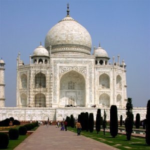
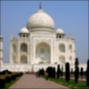
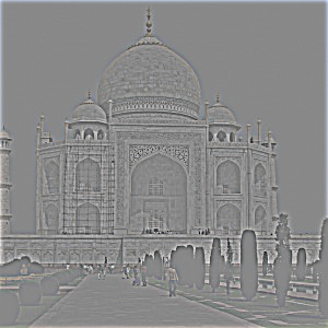
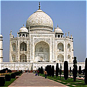
Here's an example of the technique applied to the following Taj image, using parameters \(\text{kernel size k} = 9\) and \(\text{sigma} = 2\) for the Gaussian filter and \(\alpha=2\):

As we can see, the sharpened image for the Taj image has sharper edges and a more crisp look compared to the regular Taj image.

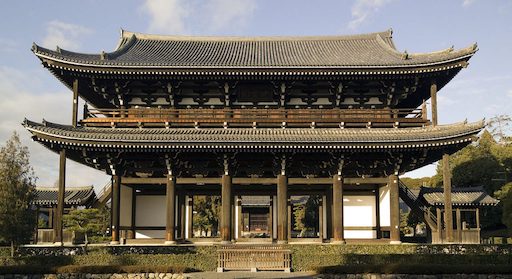
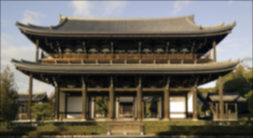
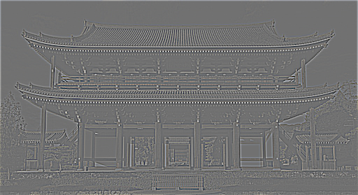
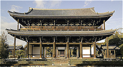
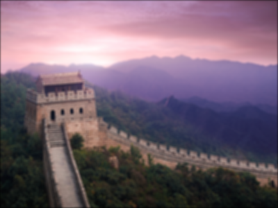
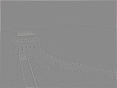
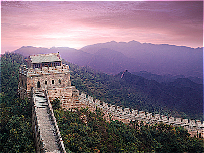
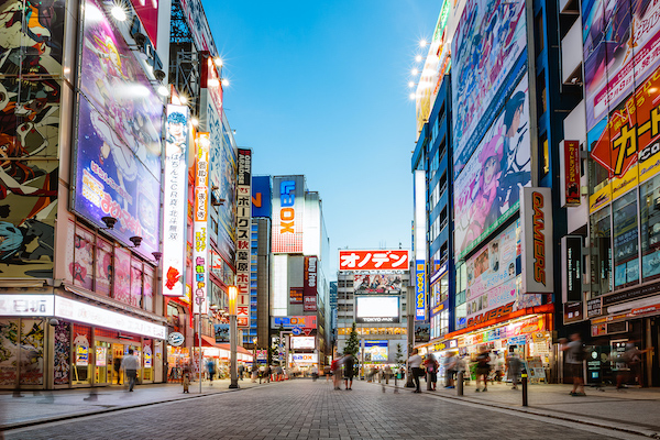
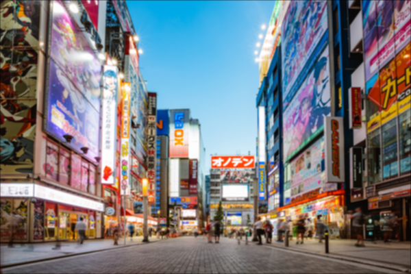
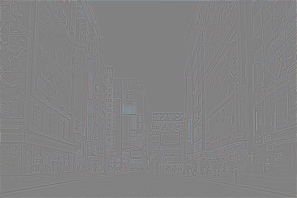
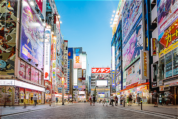
I also tried the sharpening technique on other images (Monastery, Great Wall of China, Tokyo), with parameters \(\text{kernel size k} = 9\) and \(\text{sigma} = 5\) for the Gaussian filter and \(\alpha=2\):

Part 2.2: Hybrid Images

Here, I created hybrid images by combining two images in the following manner: I take the grayscale images for both images, align the images together by taking two reference points (usually these are eyes), and then low-pass filter one image and high-pass filter another image (obtained by subtracting original image by the low-pass filtered version of the image). Finally, add the two images together in order to get the hybrid image.

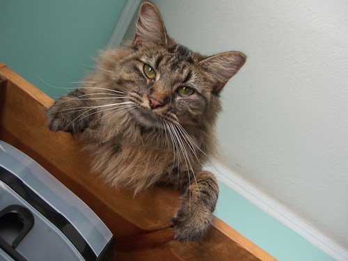
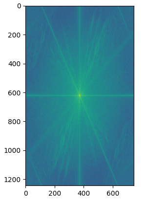
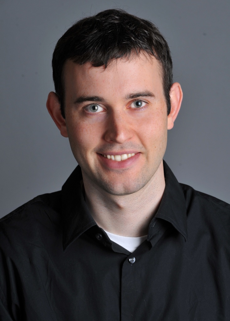
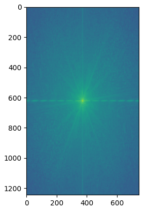
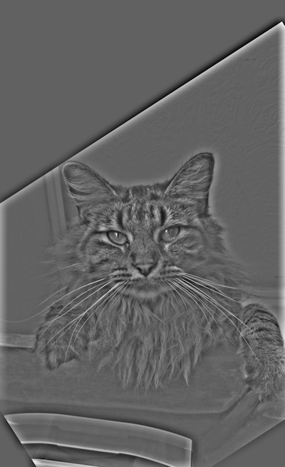
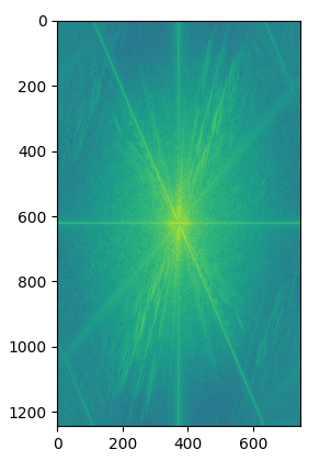
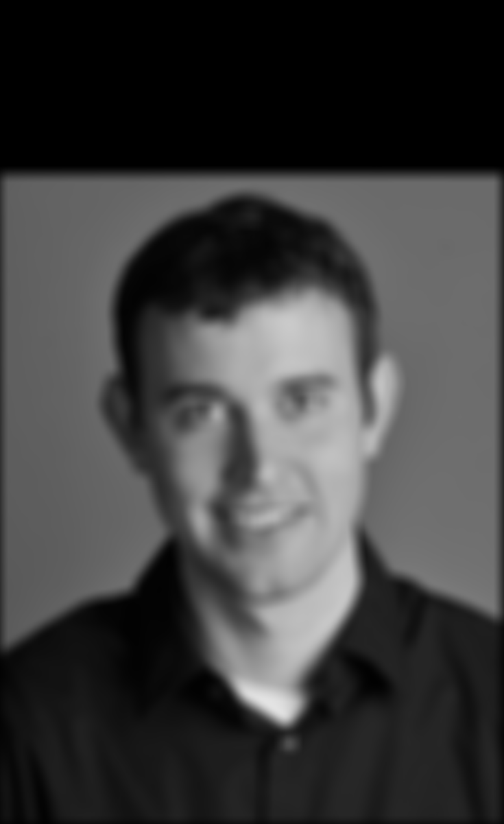
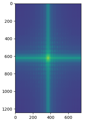
I tried the process on the images of Nutmeg and Derek. For each image involved (Nutmeg, Derek, high-pass filtered Nutmeg, low-pass filtered Derek, and the hybrid image), I also produced the 2D fourier transform for the image and displayed them underneath the image. Parameters: \(\text{kernel size k} = 40\) and \(\text{sigma} = 20\) for Gaussian filter applied to Nutmeg, \(\text{kernel size k} = 25\) and \(\text{sigma} = 10\) for Gaussian filter applied to Derek:

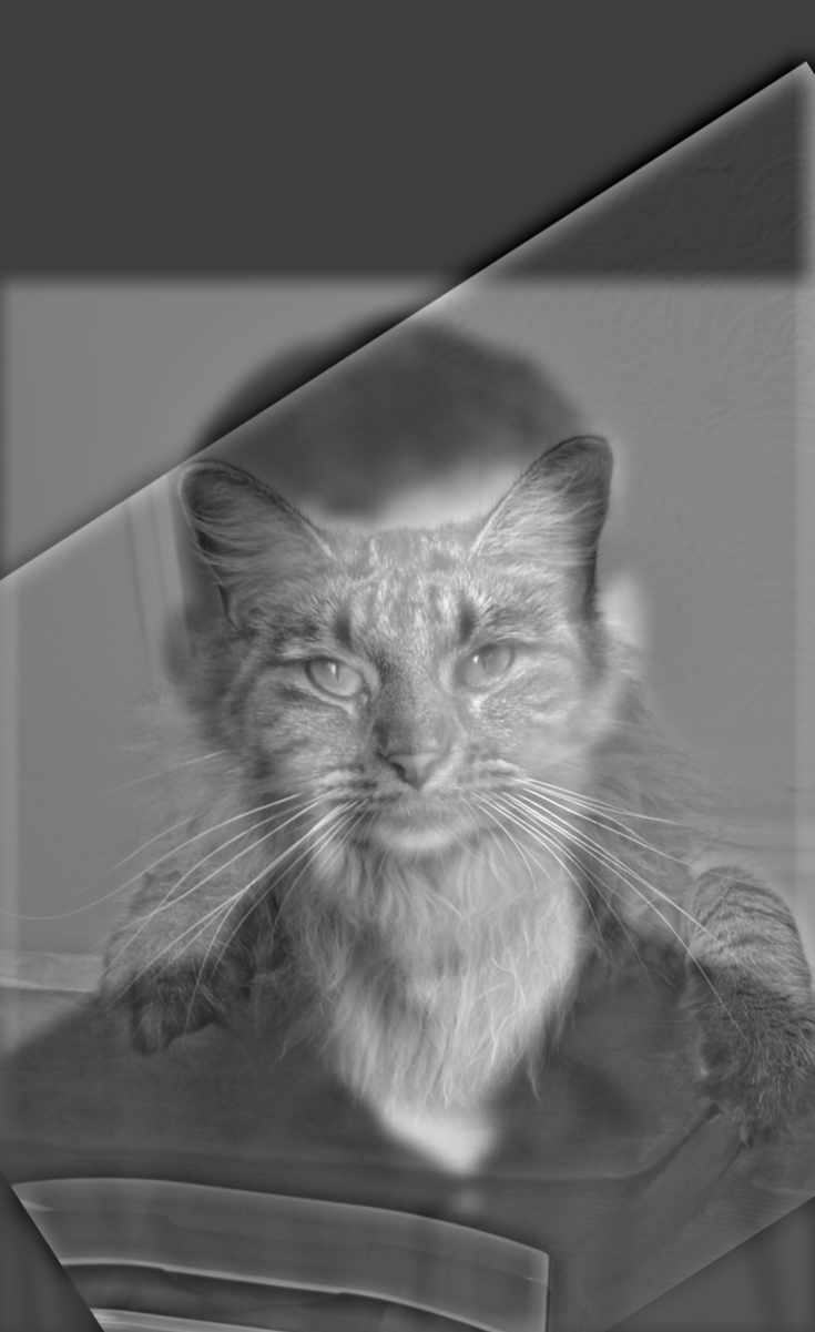
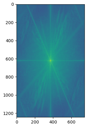
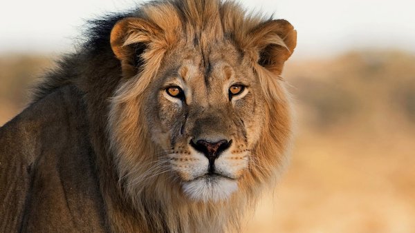
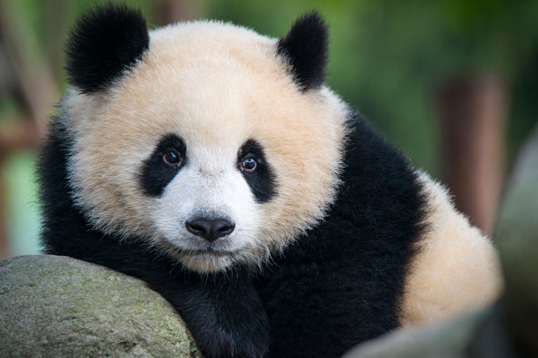
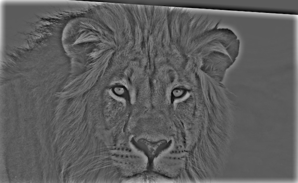
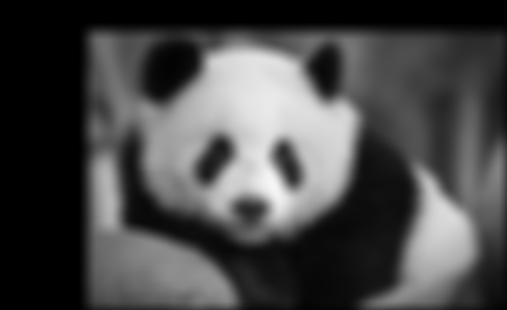
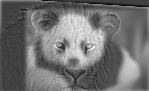
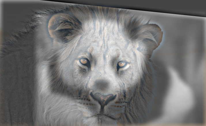
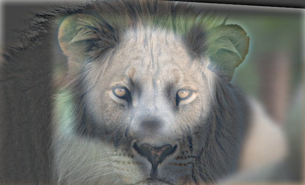
Here is another example with lion and panda as the images (Parameters: \(\text{kernel size k} = 30\) and \(\text{sigma} = 10\) for Gaussian filter applied to lion, \(\text{kernel size k} = 25\) and \(\text{sigma} = 10\) for Gaussian filter applied to panda):

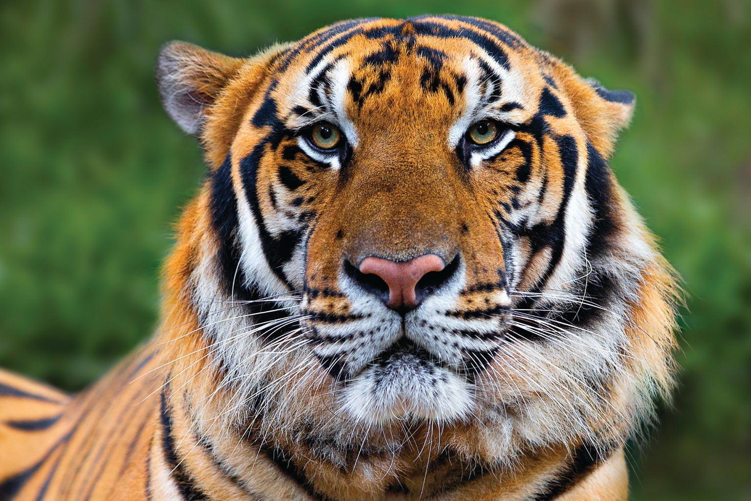
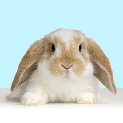
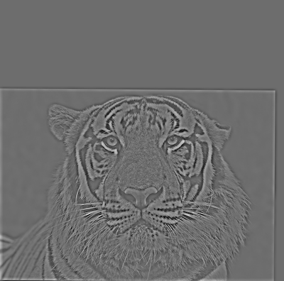
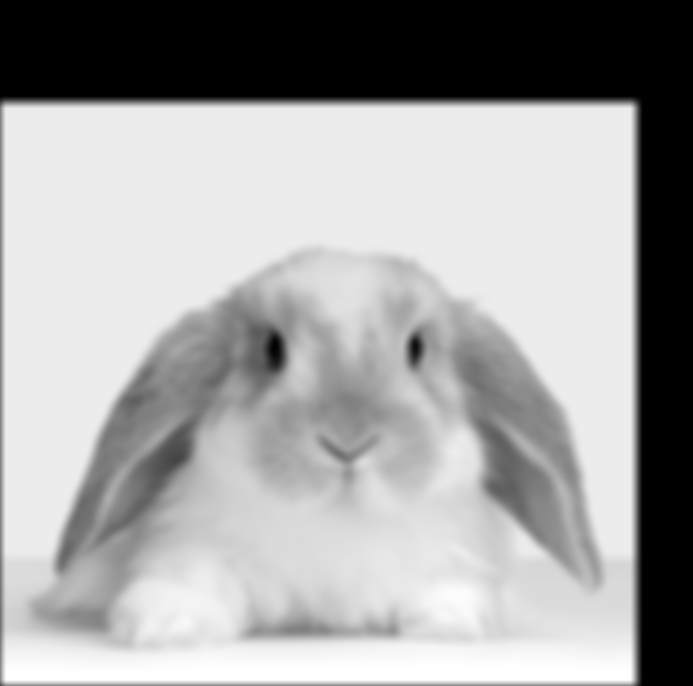
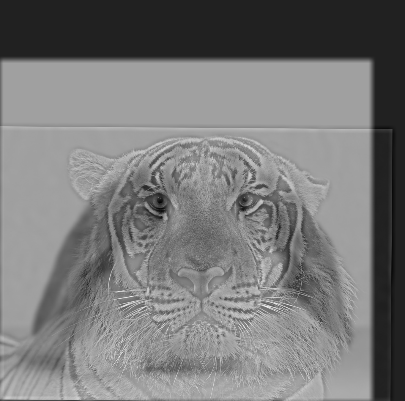
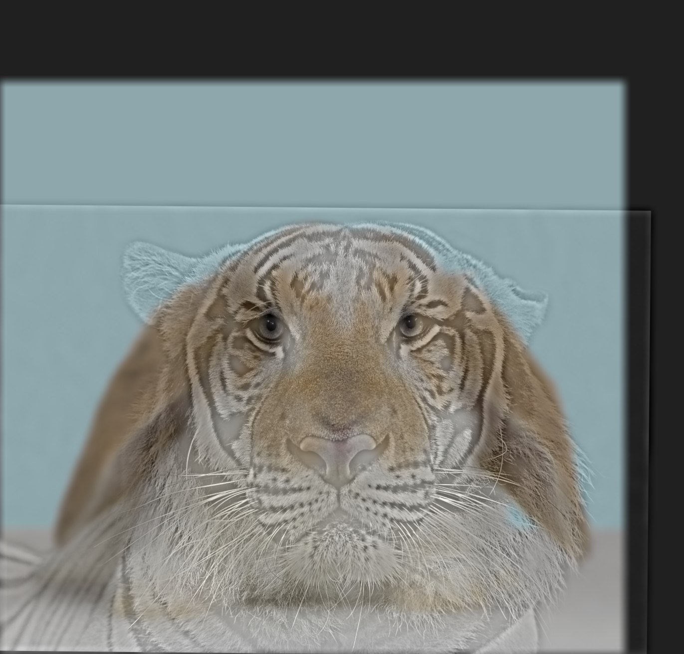
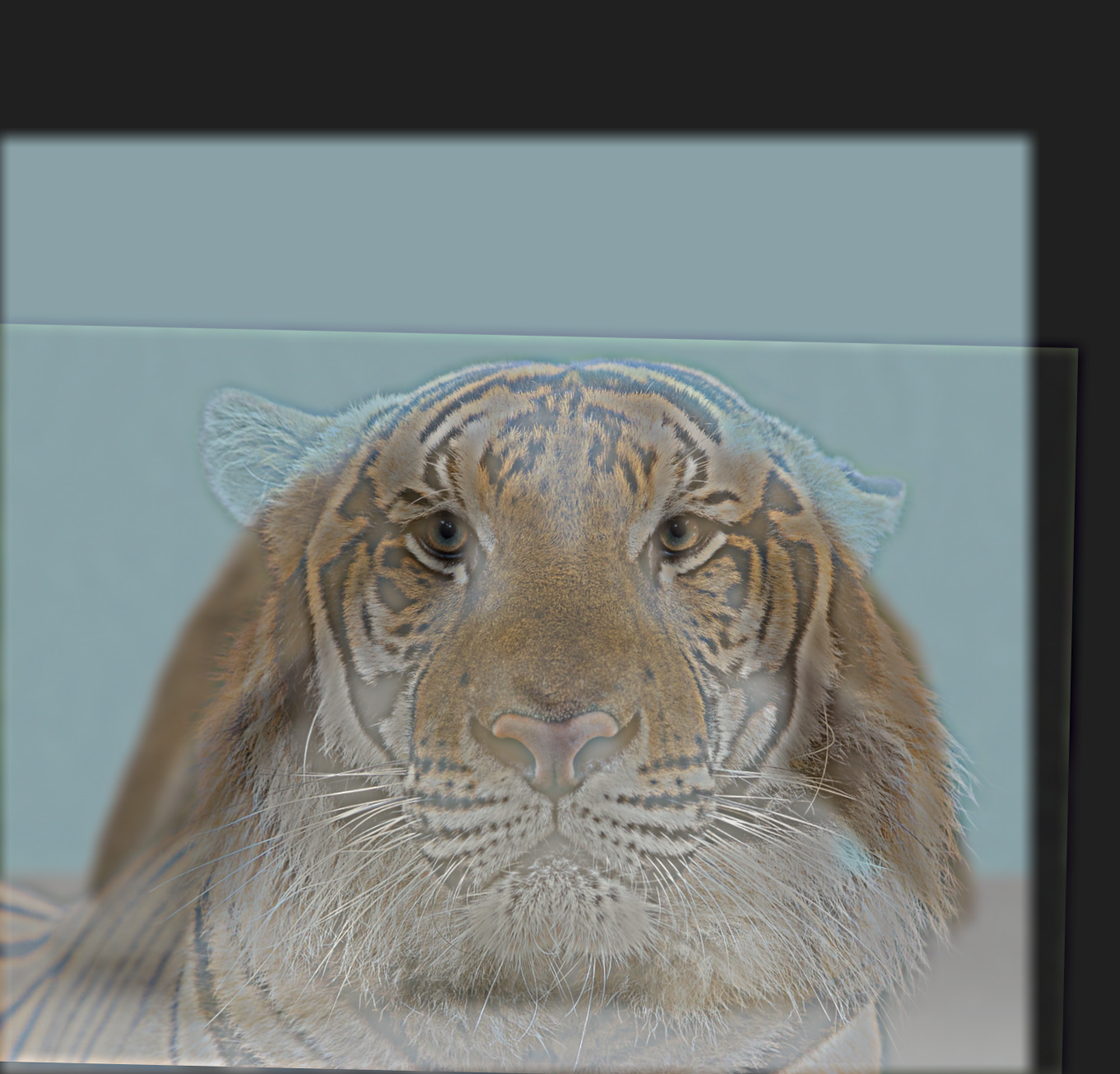
Here is another example with tiger and bunny as the images (Parameters: \(\text{kernel size k} = 30\) and \(\text{sigma} = 10\) for Gaussian filter applied to tiger, \(\text{kernel size k} = 25\) and \(\text{sigma} = 10\) for Gaussian filter applied to bunny). Note that you'd have to stand quite far away/zoom out in order to see the bunny, so this is somewhat an edge case:

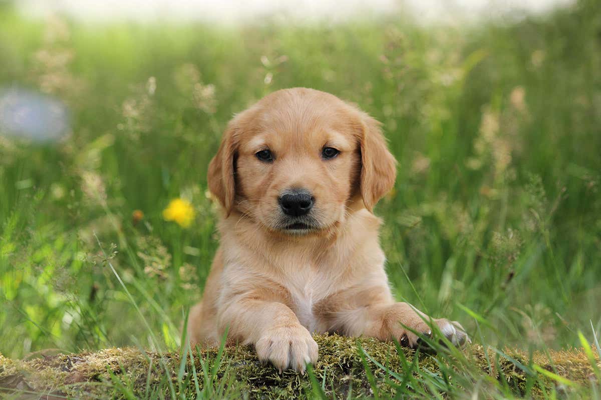
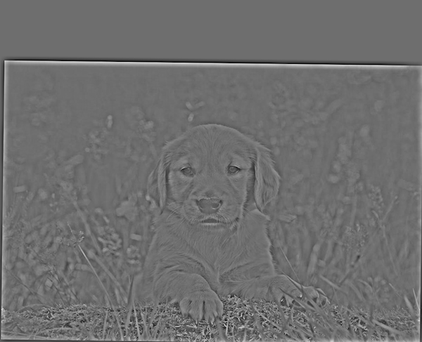
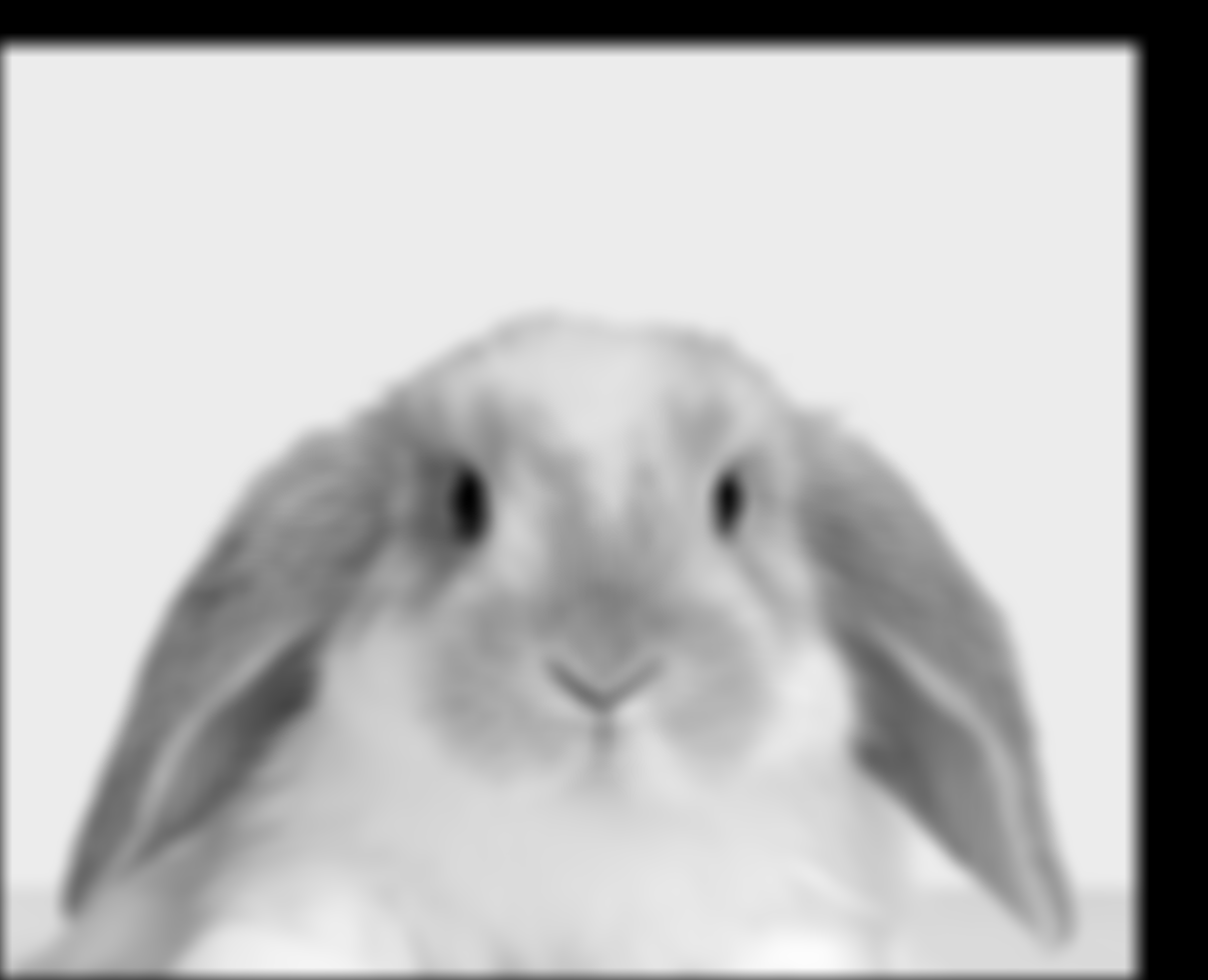
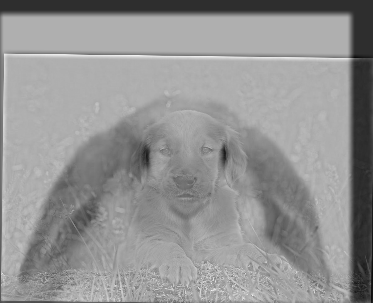
Here is a failure case example with a puppy and bunny (Parameters: \(\text{kernel size k} = 30\) and \(\text{sigma} = 10\) for Gaussian filter applied to puppy, \(\text{kernel size k} = 25\) and \(\text{sigma} = 10\) for Gaussian filter applied to bunny). When you're far away, you can see the bunny, but when you're close, you can't really see the puppy very clearly:

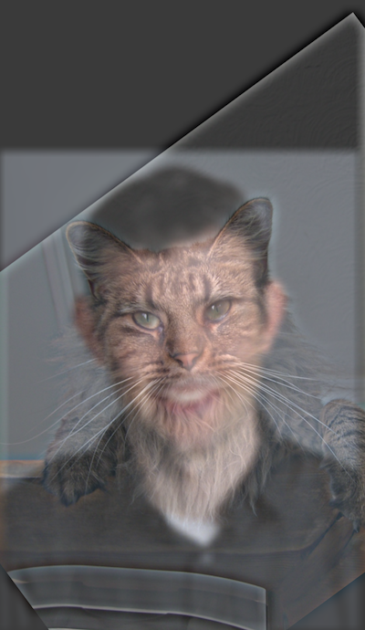
Next, I tried experimenting with color (Bells & Whistles). Some examples looked better where low pass was colored or where high pass was colored (but the rest looked worse); I've included the best looking images below. I also included the results of keeping both images colored below. I held the Gaussian filter parameters similarly to how I held them above for the respective images:

Part 2.3: Gaussian and Laplacian Stacks

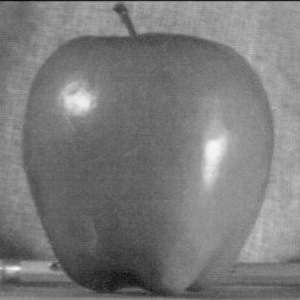
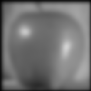
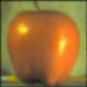
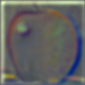
In parts 2.3 and 2.4 of the project, I work to create an oraple image through multi-resolution blending of an apple image and an orange image together. In this part, I create Gaussian and Laplacian stacks of the apple and orange images to aid in creation of the oraple image.

For the Gaussian stacks for each image, I created \(N = 10\) identical copies of the grayscale apple and orange images. Then, for each image Gaussian stack, I hold the topmost level constant, and apply a Gaussian filter with parameters \(\text{kernel size k} = 10\) and \(\text{sigma} = 5\) to the remaining \(N-1\) images in the levels below. Then, I hold the second level constant, and again applied the Gaussian filter to the remaining \(N-2\) images below. I continue this pattern until I only apply the Gaussian filter to the last level of the Gaussian stack for each image.

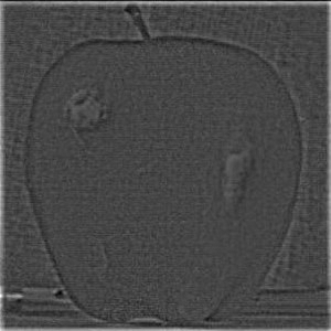
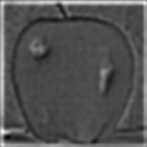
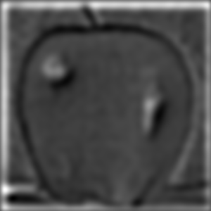
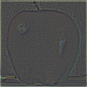
For the Laplacian stacks for each image, I take the respective Gaussian stack, and perform the following computation: laplacian_stack[i] = gaussian_stack[i] - gaussian_stack[i+1] for i in \([0,N-1)\) (0 indexed). The last level of the Laplacian stack is set to the image of the last level of the Gaussian stack, because the last level of the Laplacian stack should have lowest frequency. I normalize each image of the Laplacian stack before saving the image, using method (matrix - np.min(matrix)) / np.max(matrix) - np.min(matrix), but don't use the normalized Laplacian images in the creation of the oraple.

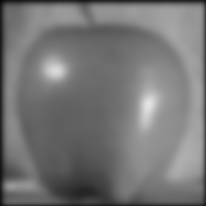
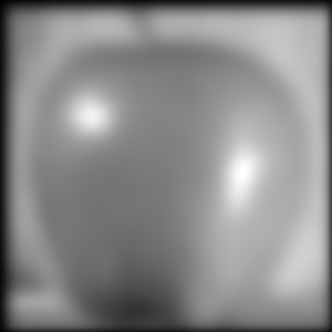
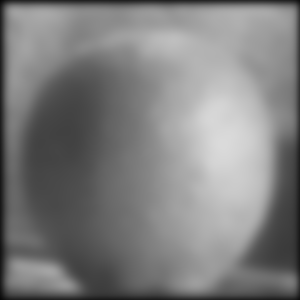
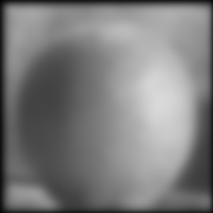
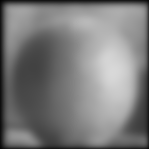
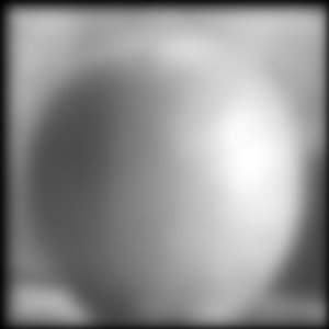
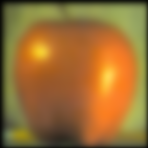
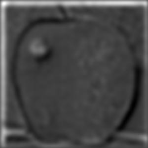
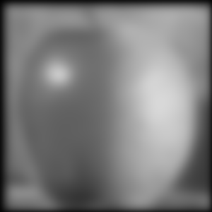
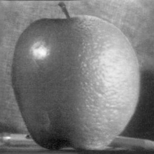
Here are images corresponding to depth 1, 3, 5, 8, 10 of the Apple Gaussian stack (1 indexed):

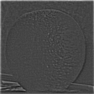
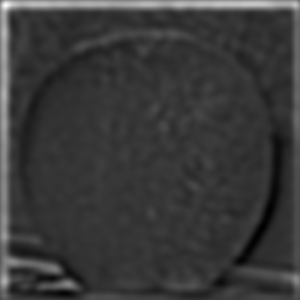
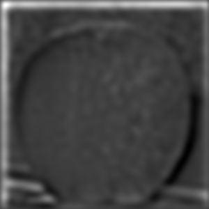
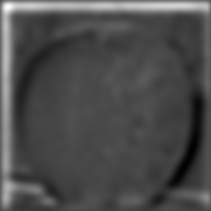
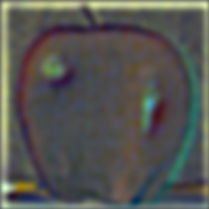
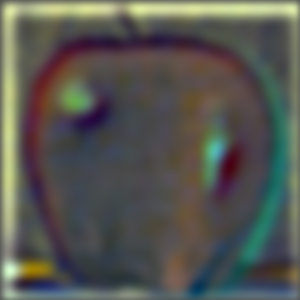
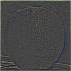
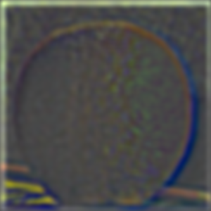
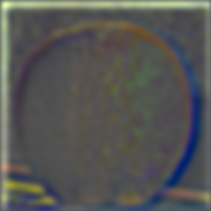
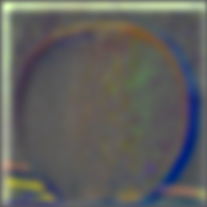
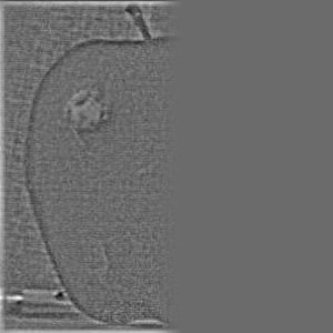
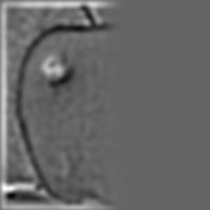
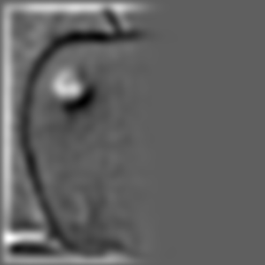
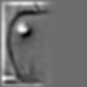
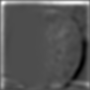
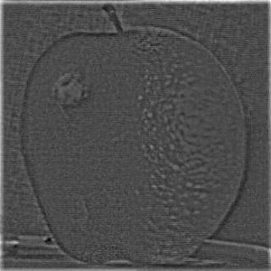
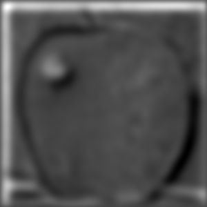
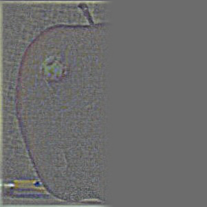
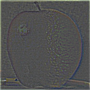
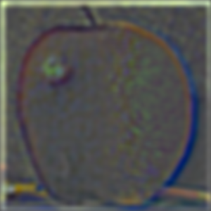
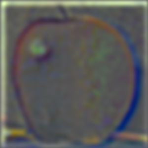
Here are images corresponding to depth 1, 3, 5, 8, 10 of the Apple Laplacian stack:

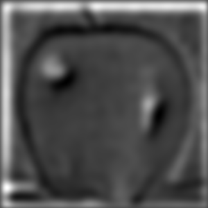
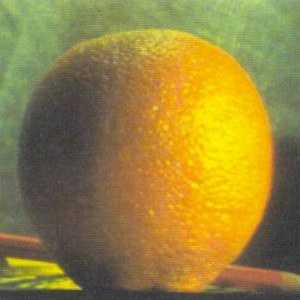
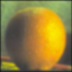
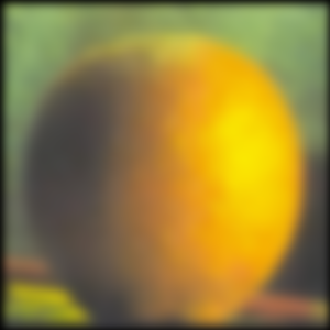
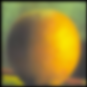
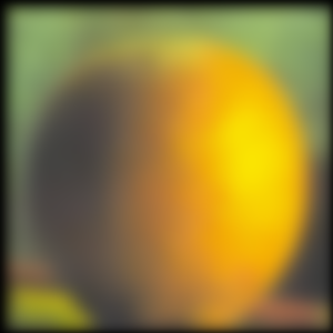
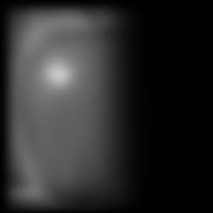
Here are images corresponding to depth 1, 3, 5, 8, 10 of the Orange Gaussian stack:

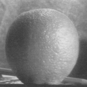
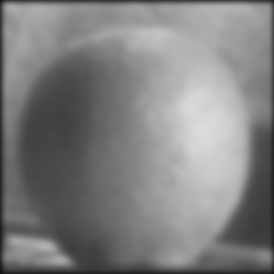
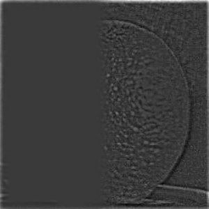
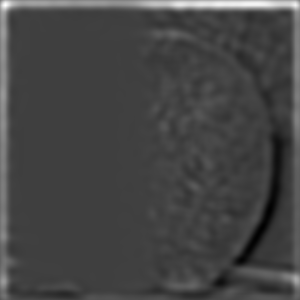
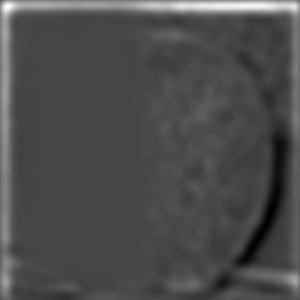
Here are images corresponding to depth 1, 3, 5, 8, 10 of the Orange Laplacian stack:

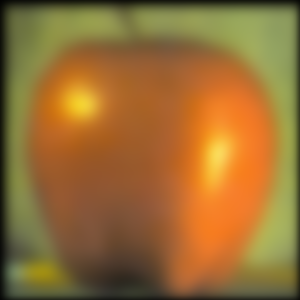
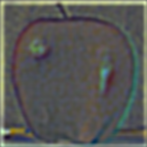
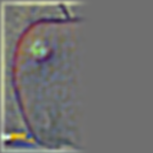
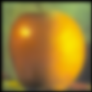
Additionally, I will show the color images too to demonstrate enhancement from color (Bells & Whistles). For the color images, I used stacks of size \(N=10\), a Gaussian filter with parameters \(\text{kernel size k} = 10\) and \(\text{sigma} = 5\) to create the Gaussian stack.

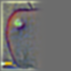
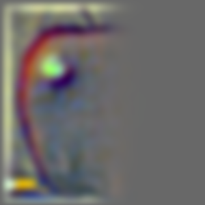
Here are images corresponding to depth 1, 3, 5, 8, 10 of the Apple (Color) Gaussian stack:

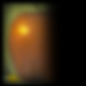
Here are images corresponding to depth 1, 3, 5, 8, 10 of the Apple (Color) Laplacian stack:

Here are images corresponding to depth 1, 3, 5, 8, 10 of the Orange (Color) Gaussian stack:

Here are images corresponding to depth 1, 3, 5, 8, 10 of the Orange (Color) Laplacian stack:

Part 2.4: Multiresolution Blending

In parts 2.3 and 2.4 of the project, I work to create an oraple image through multi-resolution blending of an apple image and an orange image together. In this part, I use the Gaussian and Laplacian stacks from part 2.3 in order to blend the two images together seamlessly.

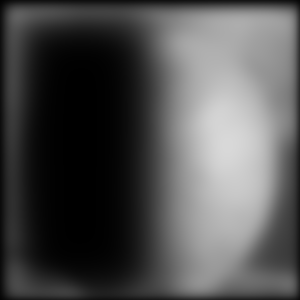
I create a mask that is a NumPy array that has the same dimension as the Apple/Orange images. I set the left half (first half of columns; axis 1) of the NumPy mask's values to 1s, and leave the rest as 0. I create a total of \(N=10\) copies of the mask, in a similar fashion to the number of levels of the Gaussian/Laplacian stacks mentioned above. I use a Gaussian filter with parameters \(\text{kernel size k} = 30\) and \(\text{sigma} = 10\), and follow a similar procedure of applying the Gaussian filter to the levels of the mask stack as I did when creating the Gaussian stacks for the apple and orange. This mask will be helpful for computing the output image for the oraple. An image of the mask is attached below:

I use the following algorithm to compute the output image: out += mask_stack[i] * im1_laplacian_stack[i] + (1 - mask_stack[i]) * im2_laplacian_stack[i] for i in \([0, N)\) (0 indexed), where im1 is the apple image and im2 is the orange image. I also normalize the final output before saving.

Here are images corresponding to the left half apple images (mask_stack[i] * im1_laplacian_stack[i]) for depths 1, 3, 5, 8, 10 (1 indexed):

Here are images corresponding to the right half orange images ((1 - mask_stack[i]) * im2_laplacian_stack[i]) for depths 1, 3, 5, 8, 10:

Here are images corresponding to the combined image (mask_stack[i] * im1_laplacian_stack[i] + (1 - mask_stack[i]) * im2_laplacian_stack[i]) at depths 1, 3, 5, 8, 10:

Here is the final oraple:

Additionally, I will show the color images too to demonstrate enhancement from color (Bells & Whistles). I use \(N = 10\) for the size of the mask stack, and use a Gaussian filter with parameters \(\text{kernel size k} = 30\) and \(\text{sigma} = 10\).

Here are images corresponding to the left half apple (color) images (mask_stack[i] * im1_laplacian_stack[i]) for depths 1, 3, 5, 8, 10:

Here are images corresponding to the right half orange (color) images ((1 - mask_stack[i]) * im2_laplacian_stack[i]) for depths 1, 3, 5, 8, 10:

Here are images corresponding to the combined (color) image (mask_stack[i] * im1_laplacian_stack[i] + (1 - mask_stack[i]) * im2_laplacian_stack[i]) at depths 1, 3, 5, 8, 10:

Here is the final oraple (color):

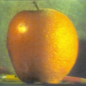
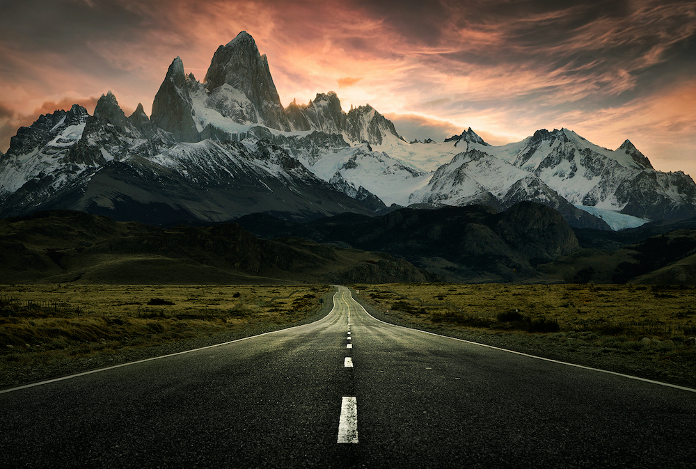
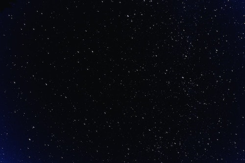
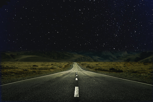
I also experimented with multiresolution blending on other additional images. I blended an image of road/mountain scenery with the night sky, using a mask with the top half of the image as 0s and the bottom half of image as 1s. I use \(N = 8\) levels for the stacks. For the Gaussian stacks I used parameters \(\text{kernel size k} = 20\) and \(\text{sigma} = 5\); for the mask Gaussian stack I used parameters \(\text{kernel size k} = 10\) and \(\text{sigma} = 20\).

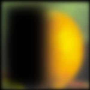
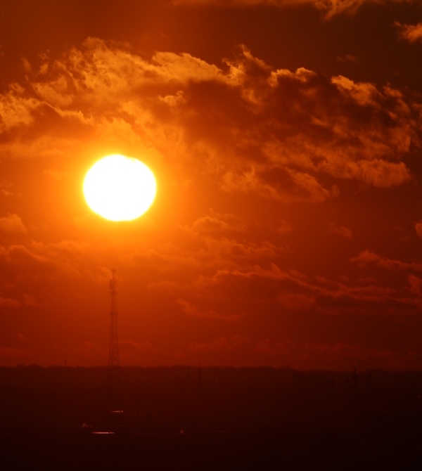
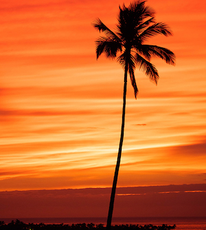
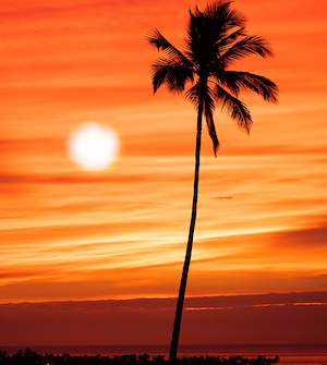
I blended an image of palm tree + sky scenery with an image of a sun, using a irregularly-shaped mask where areas outside of the sun are 0s and the areas approximately inside the sun are 1s. I use \(N = 8\) levels for the stacks. For the Gaussian stacks I used parameters \(\text{kernel size k} = 20\) and \(\text{sigma} = 5\); for the mask Gaussian stack I used parameters \(\text{kernel size k} = 10\) and \(\text{sigma} = 20\).

Summary

I learned about how to apply filters to images to extract different frequencies / features and then combine various forms of images (regular image, low-pass filtered image, high-pass filtered image) in ways that makes the images sharper or smoother (for blending). The most important thing I learned from this project was multiresolution blending, which taught me how to apply muliple filtering techniques for two images in a way that produces a smooth, elegantly-blended final image. It allowed me to tackle challenges and explore creativity in choosing what images to combine, fine tuning Gaussian filters, creating masks (and in some cases, irregular-shaped masks), and combining images to create the final image.

Acknowledgements

• CS194-26 Project Description and Starter Project Code(For Hybrid Image)
• I've obtained the Cameraman, Taj, Nutmeg, Derek Picture, Apple, and Orange pictures from CS194-26 Starter Project Code.
• I've obtained the following images from Google search (using exact/similar terms stated): Chinese Monastery, Great Wall of China, Tokyo, Lion, Panda, Tiger, Bunny, Puppy, Road Mountains Picture, Night Sky, Sun, Palm Tree