Section 1.1: Fun with Filters - Finite Difference Operator
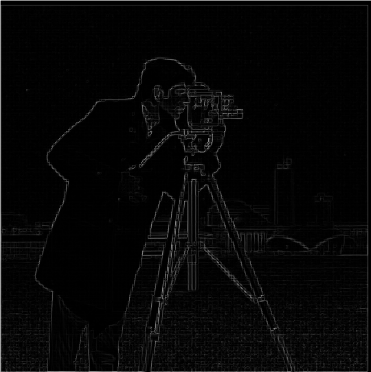
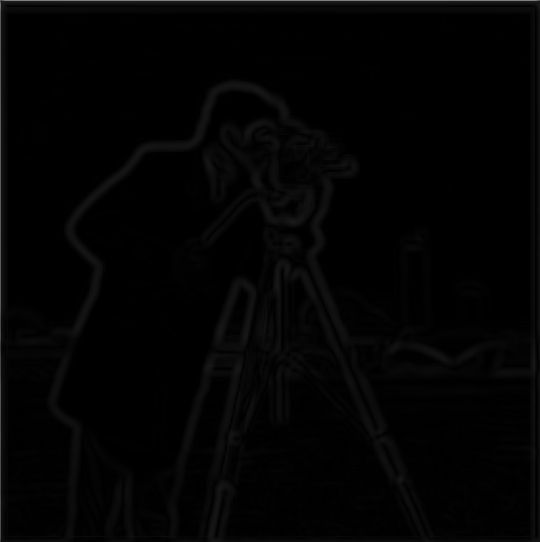
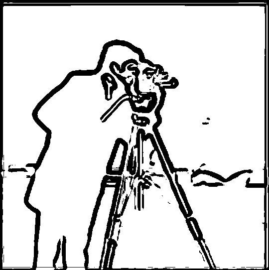
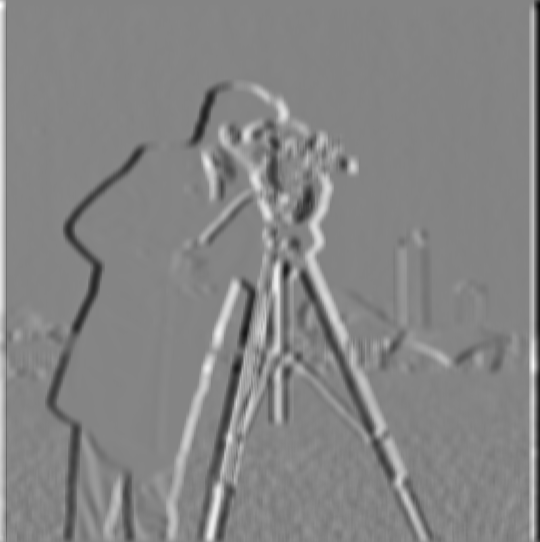
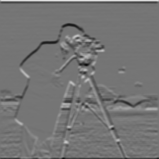
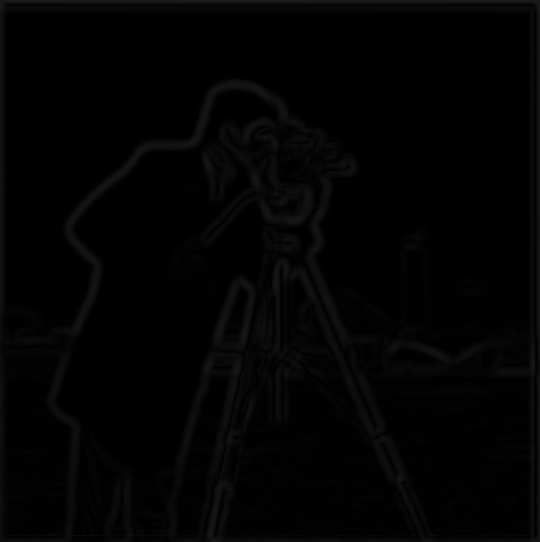
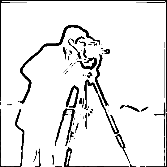
In this first part of the project, I computed an estimate of the partial derivatives with respect to X and Y by convolving the original image with the finite difference operators [1, -1] and its transpose (D_x and D_y respectively). In order to compute the gradient magnitude, I simply performed an element-wise square of the elements of each partial derivative (w.r.t x and y) of the original image, added the squared matrices together, and took the element-wise square root of the sum. Finally, I compared each element within the gradient magnitude matrix in order to binarize the image and visualize the edges.
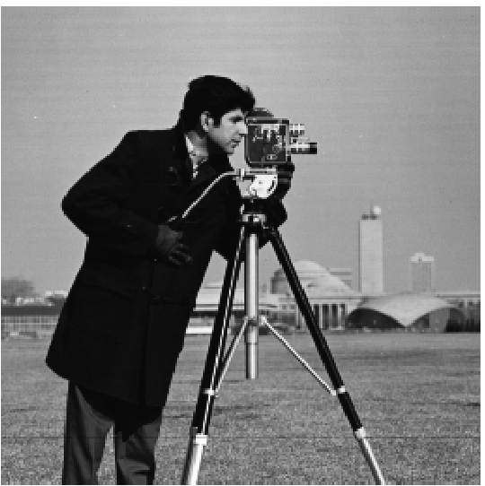 Original Image: cameraman.png
|
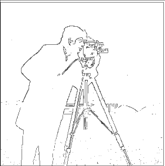 Edge Image
|
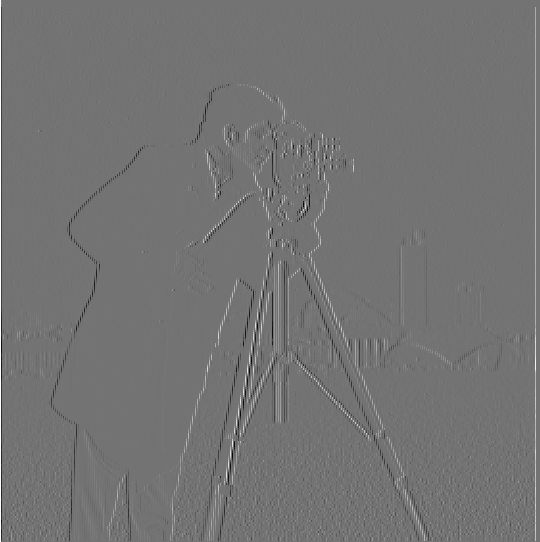 Partial Derivative w.r.t X
|
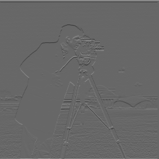 Partial Derivative w.r.t Y
|
 Gradient Magnitude
|
Section 1.2: Fun with Filters - Derivative of Gaussian (DoG) Filter
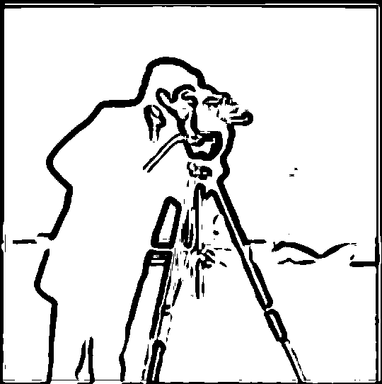
By utilzing a Gaussian filter (a low pass filter), we allow lower frequencies within the image to pass through while discarding higher frequencies. This reduces our partial derivative, gradient magnitude, and edge imags' susceptibility to noise. As you can see below, by applying our gaussian filter, less graininess is present in non-edge portions of the image and the edges are smoother. Additionally, since convolving using a Gaussian leads to averaging a pixel using nearby pixels, our edges seem to be thicker and smoother due to the lack of abrupt changes in the image.
|
Original Image: cameraman.png
|
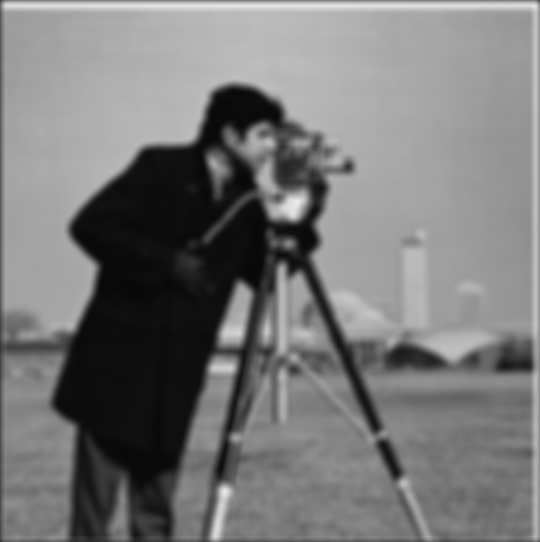 Blurred Image using Gaussian Filter
(size = 12x12, sigma = 4)
|
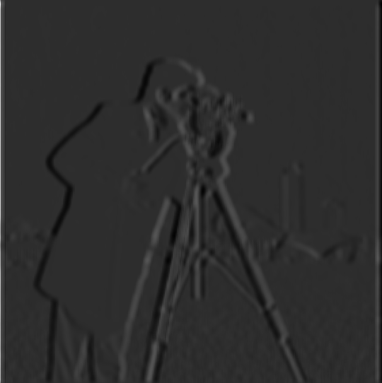 Partial Derivative w.r.t X (with Gaussian Filter)
|
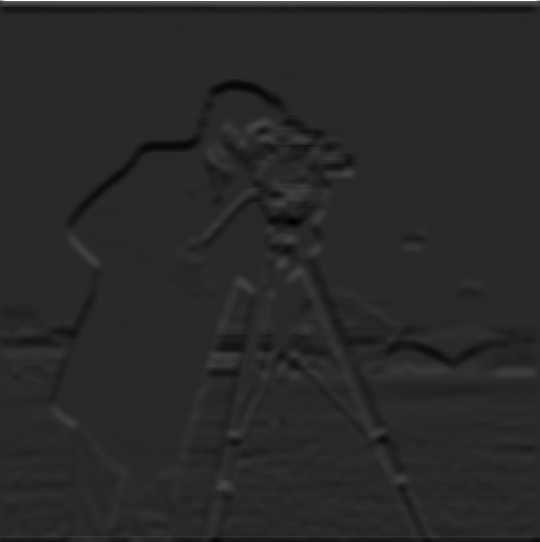 Partial Derivative w.r.t Y (with Gaussian Filter)
|
 Gradient Magnitude (with Gaussian Filter)
|
 Edge Image (threshold = 0.025)
|
 Edge Image (threshold = 0.03)
|
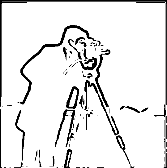 Edge Image (threshold = 0.04)
|
Additionally, instead of doing two separate convolutions on the original image(convolving when we apply a gaussian filter on the original image and again when we compute the gradients), we can convolve the gaussian with D_x and D_y and directly apply them onto the original image (one convolution), leading to the same outcome as before (just more efficient!).
 Derivative of Gaussian w.r.t X
(size = 12x12, sigma = 4)
|
 Derivative of Gaussian w.r.t Y
(size = 12x12, sigma = 4)
|
 Partial Derivative w.r.t X (with Gaussian Filter)
|
 Partial Derivative w.r.t Y (with Gaussian Filter)
|
 Gradient Magnitude (with Gaussian Filter)
|
 Edge Image (threshold = 0.04)
|
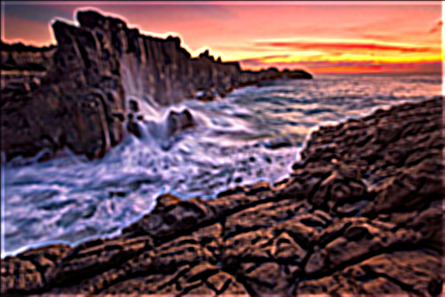
Section 2.1: Fun with Frequencies! - Image "Sharpening"
In this part of the project, I sharpened images by deriving the unsharp masking technique. In order to do this, I first scaled up the frequencies resulting from the difference between the original image and a blurred version of it (computed using a gaussian low pass filter), varying alpha (the scaling factor). Then, I derived an equivalent single convolution, called the unsharp mask filter. In other words, the unsharp mask filter adds more high frequencies to the image.
 Original Image (alpha = 0)
|
 Sharpened Image (alpha = 1)
|
 Sharpened Image (alpha = 5)
|
 Original Image (alpha = 0)
|
 Sharpened Image (alpha = 1)
|
 Sharpened Image (alpha = 5)
|
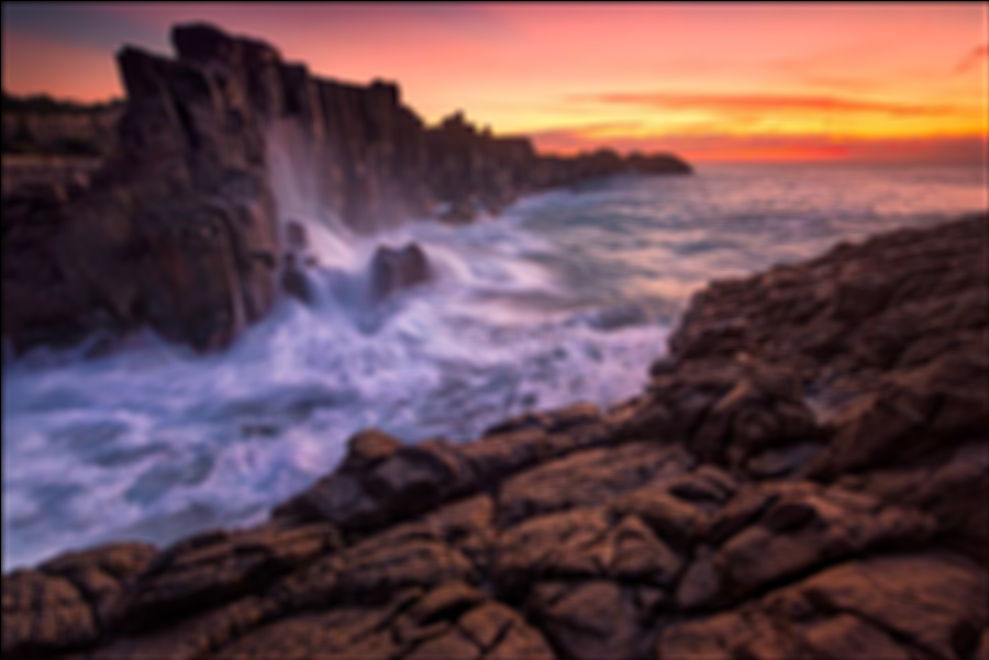
When we blur an image that was initially sharp and attempt to sharpen it again, it fails to recover the original image as the high frequencies that were present in the image before are now lost For example, the fine grains and crevasses in the rocks by the water are gone, as well as most of the mist above the water.
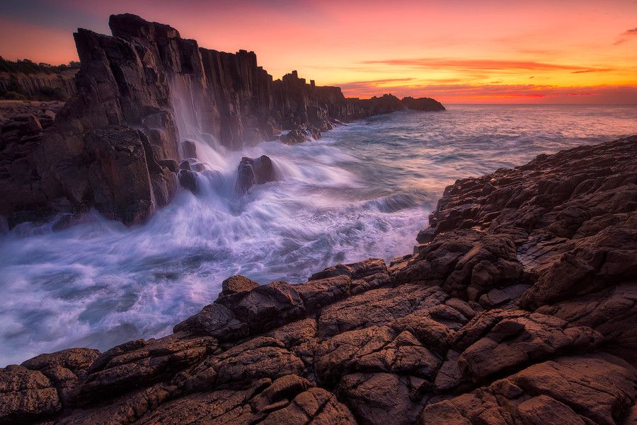 Original Image (alpha = 0)
|
 Blurred Image (Gaussian Blur)
|
 Blurred Image Sharpened (alpha = 1)
|
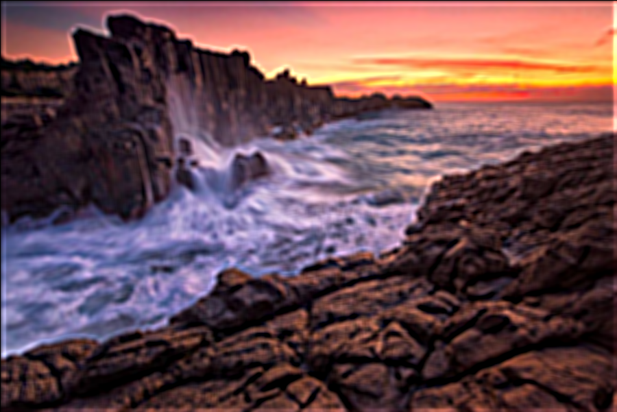 Blurred Image Sharpened (alpha = 5)
|
 Blurred Image Sharpened (alpha = 10)
|
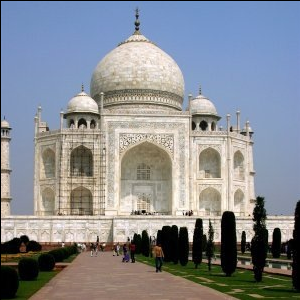
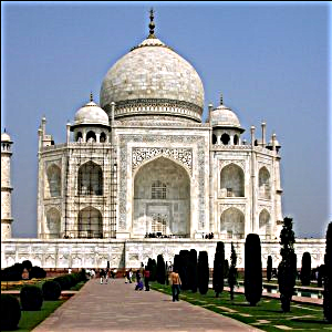
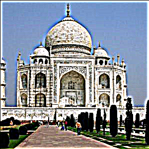
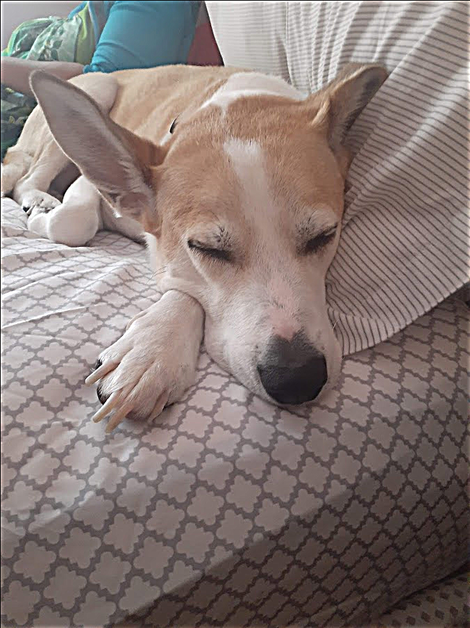
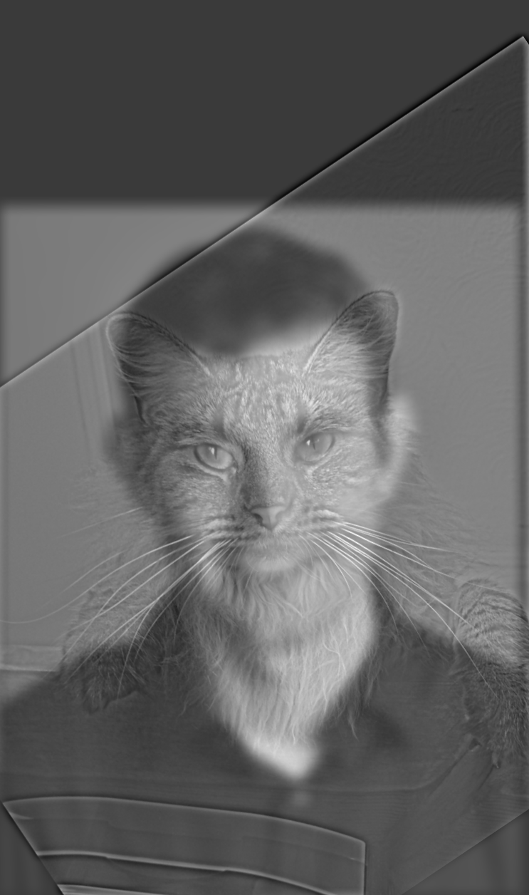
Section 2.2: Fun with Frequencies! - Hybrid Images
In this part of the project, we applied both low pass and high pass filters to two different images in order to create a hybird image. A hybrid image is a static image that changes in interpretation as a function of the viewing distance. In other words, the high frequency tends to dominate perception when it is available, but, at a distance, only the low frequency (smooth) part of the signal can be seen. By blending the high frequency portion of one image with the low-frequency portion of another, you get a hybrid image that leads to different interpretations at different distances. For retrieving the high frequencies, I am simply subtracting a blurred, low-pass version of the image from the original image. Additionally, for retrieving the low frequencies, I am using a Gaussian filter on the original image.
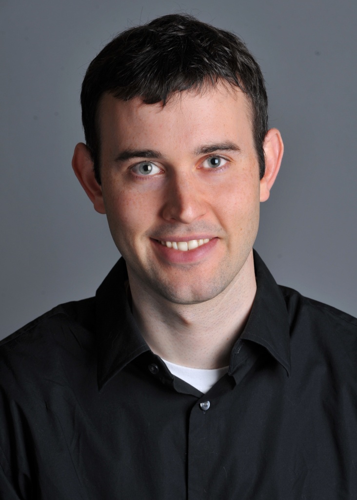 Derek
Derek
|
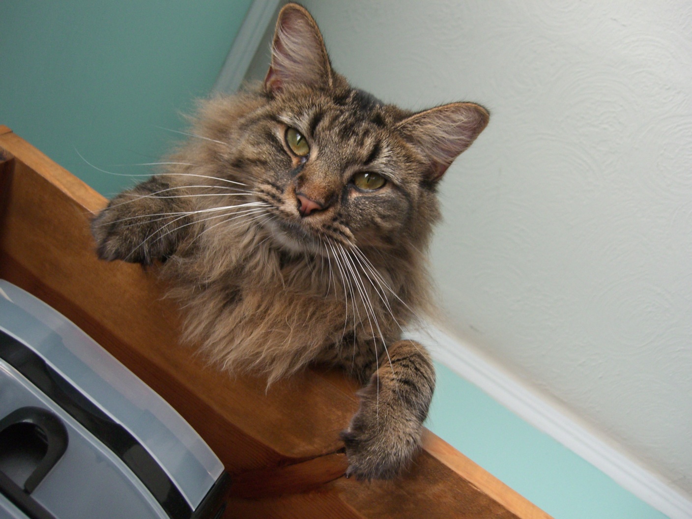 Nutmeg the Cat
|
 Low Frequency Image
(far away; Gaussian Blur applied)
|
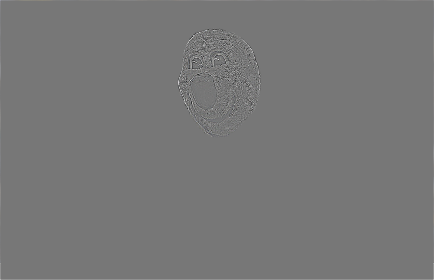
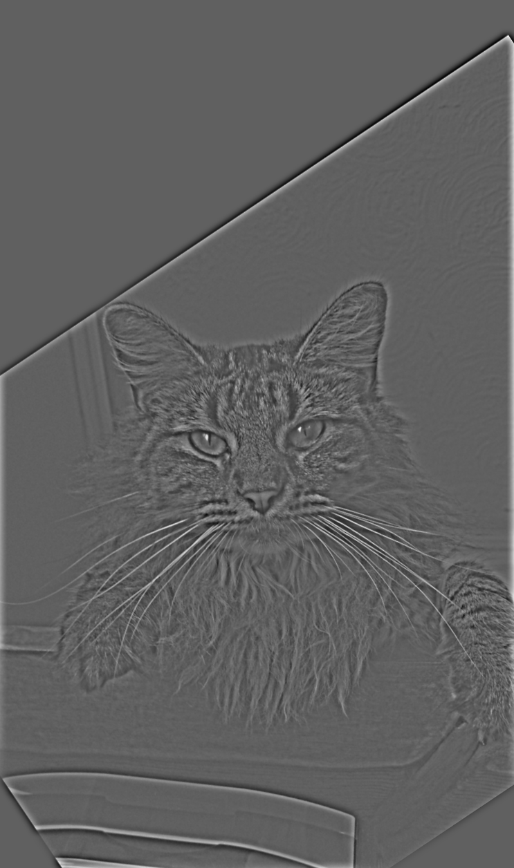 High Frequency Image (close up)
|
 Hybrid Image
|
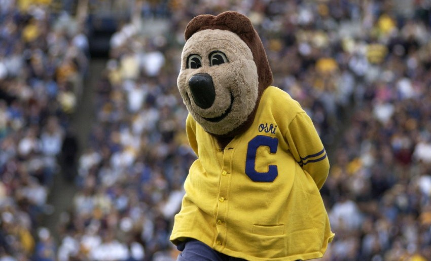
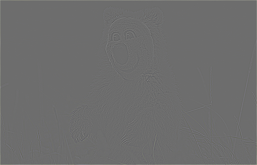
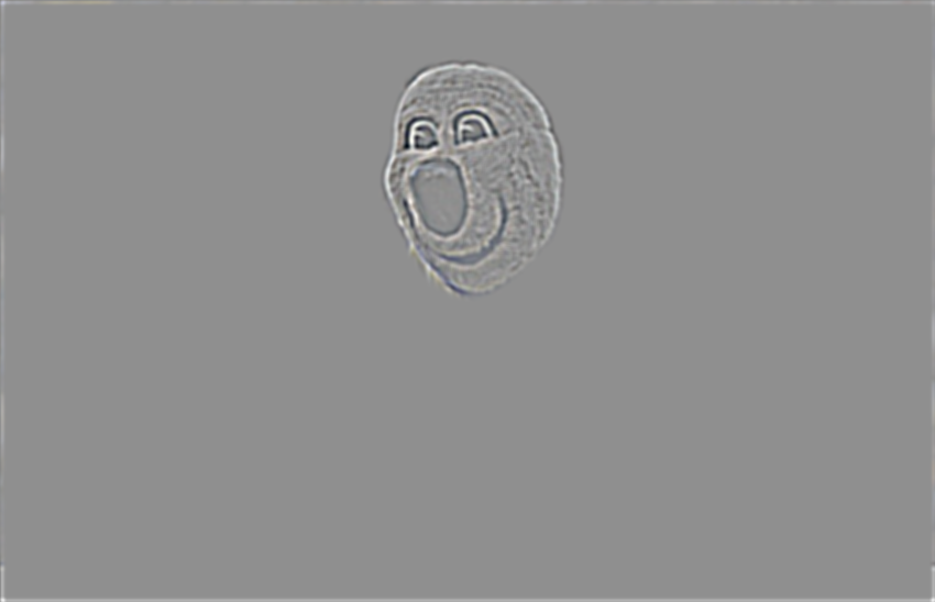
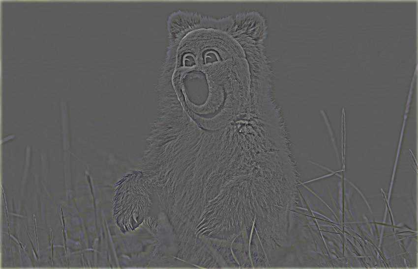
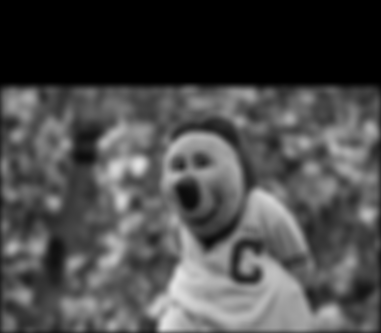
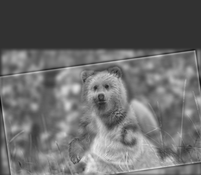
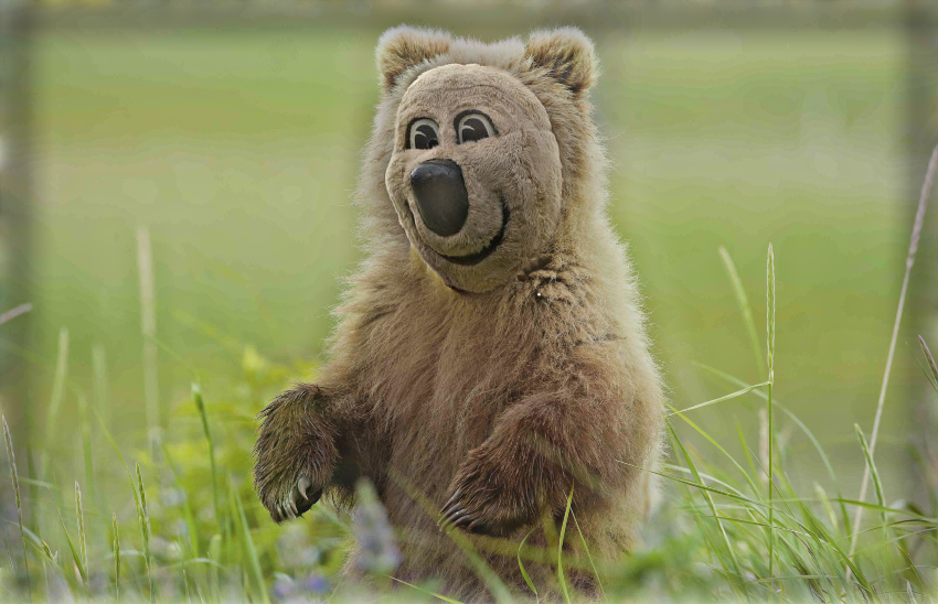
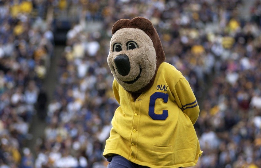 Oski
Oski
|
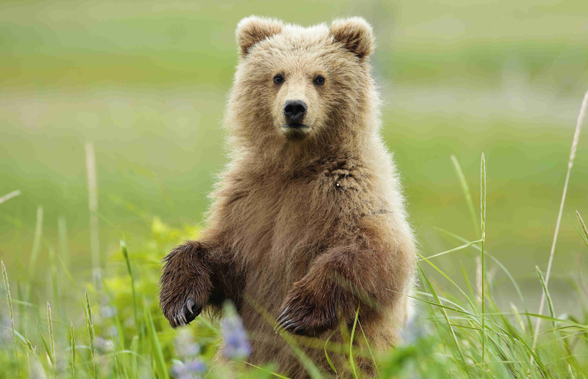
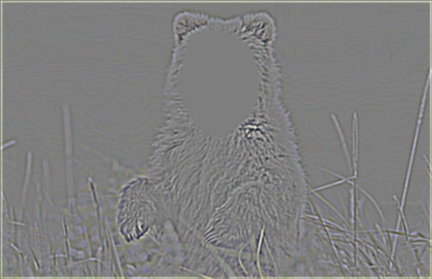
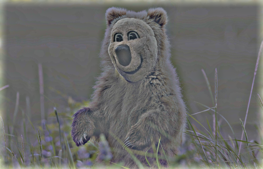
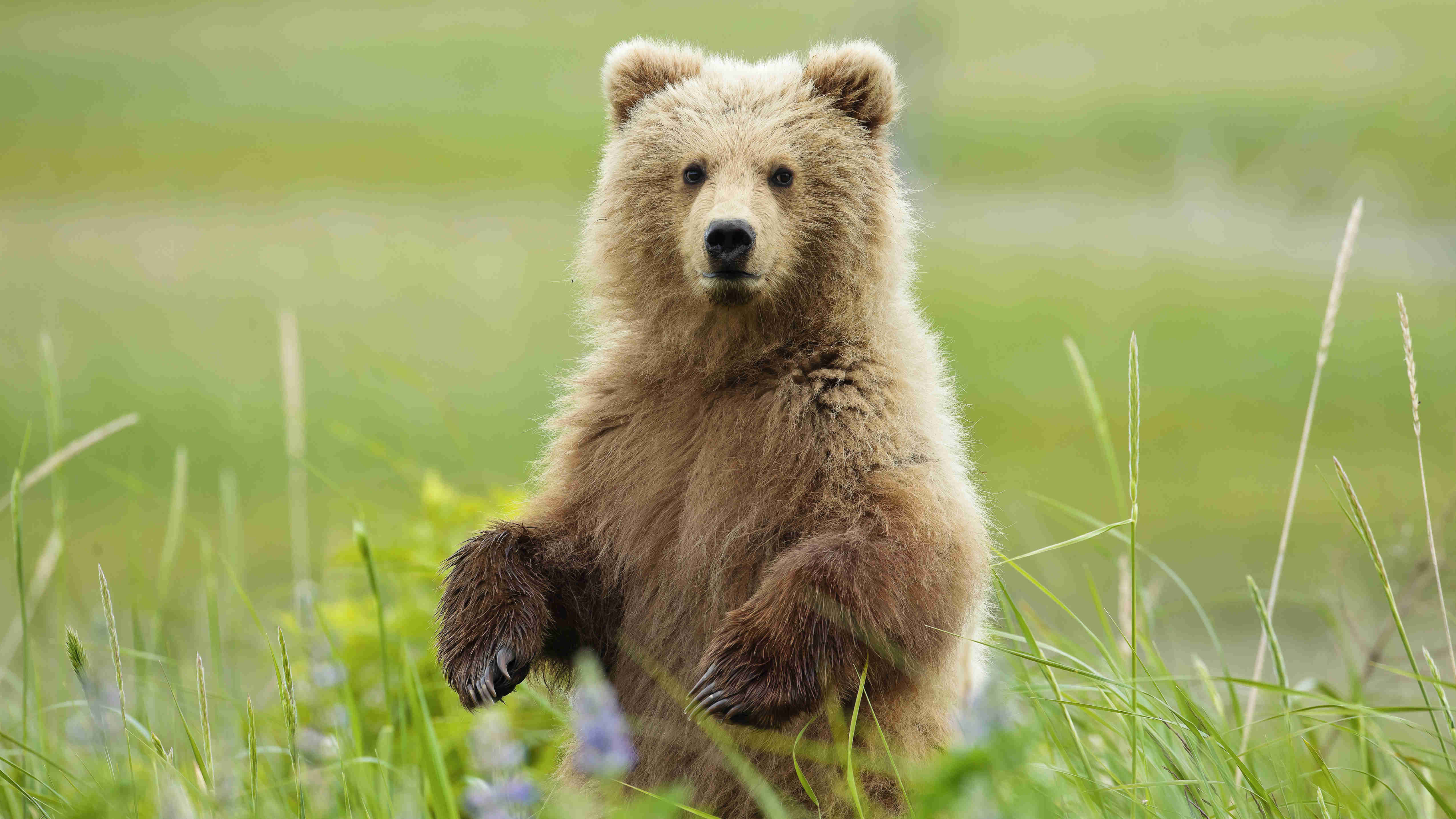 Bear
Bear
|
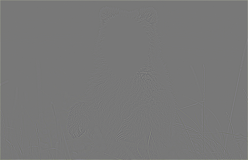
 Low Frequency Image
(far away; Gaussian Blur applied)
|
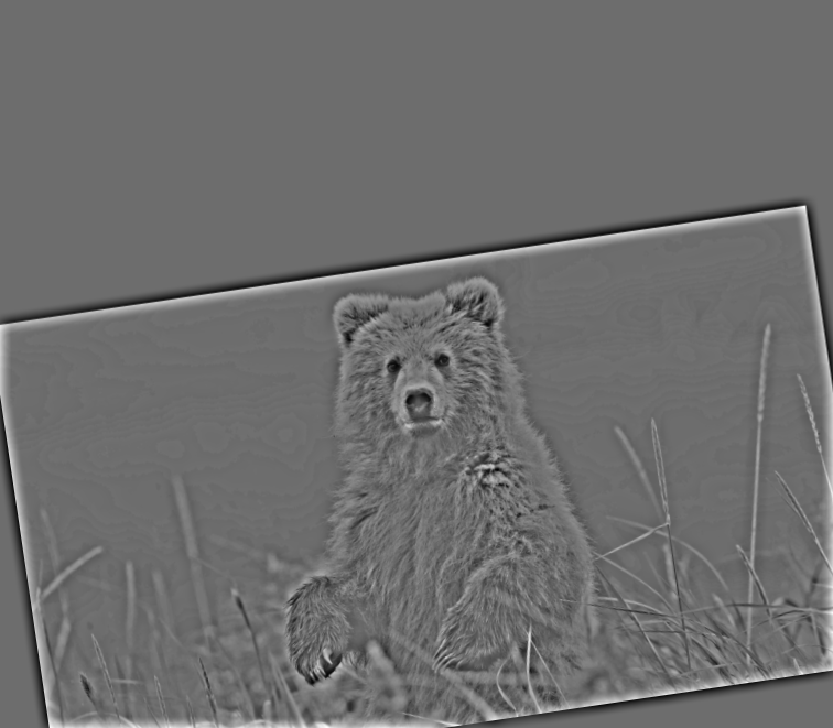 High Frequency Image (close up)
|
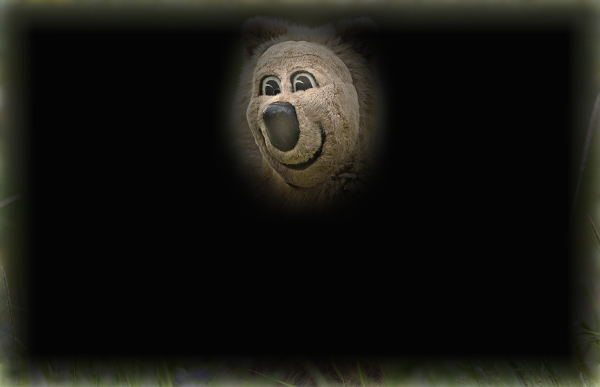
 Hybrid Far Away
|
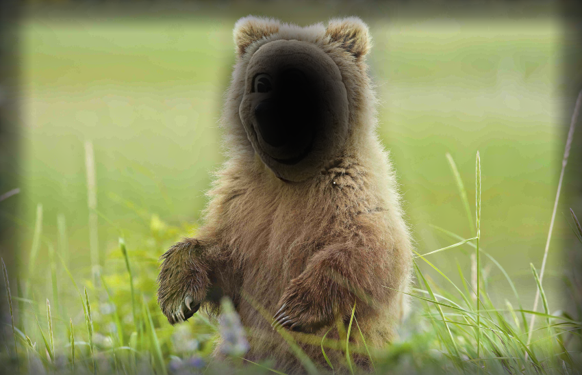
Hybrid Close Up (Zoom in for better experience)
|
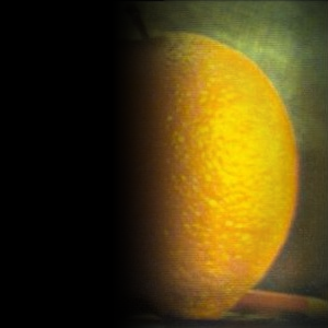
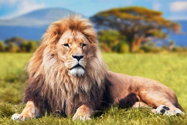
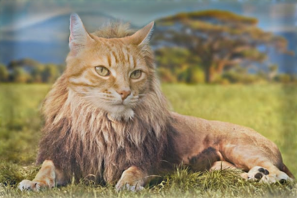
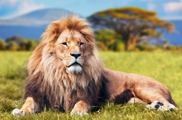 Lion
Lion
|
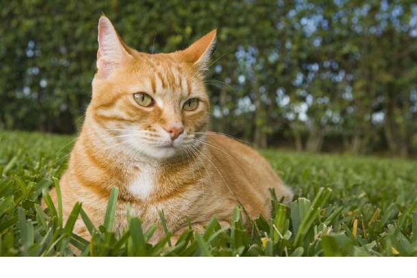
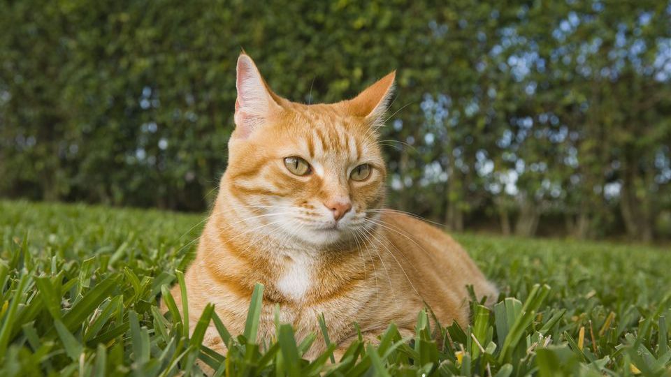 Cat
Cat
|
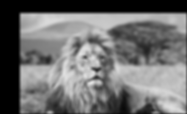 Low Frequency Image
(far away; Gaussian Blur applied)
|
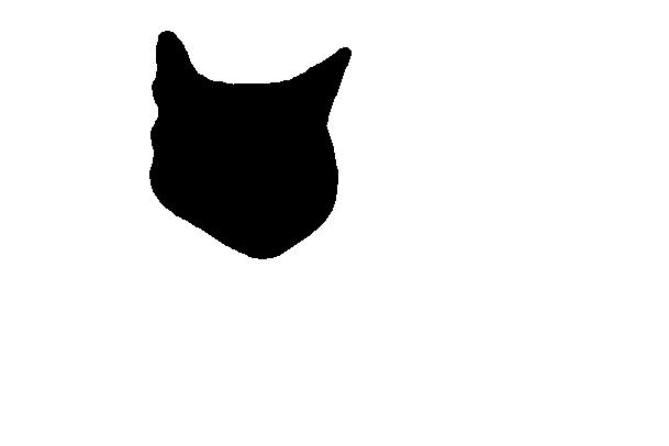
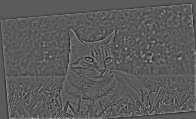 High Frequency Image (close up)
|
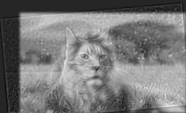 Hybrid Far Away
|
Hybrid Close Up (Zoom in for better experience)
|
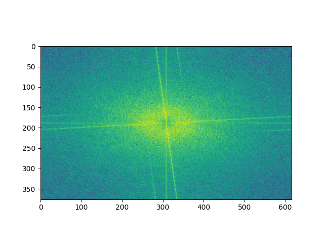
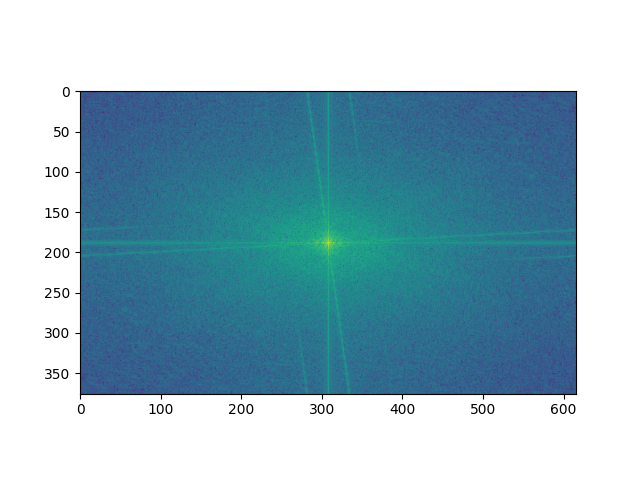
Frequency Analysis for LionCat:
 Lion Before Low-Pass Filter
|
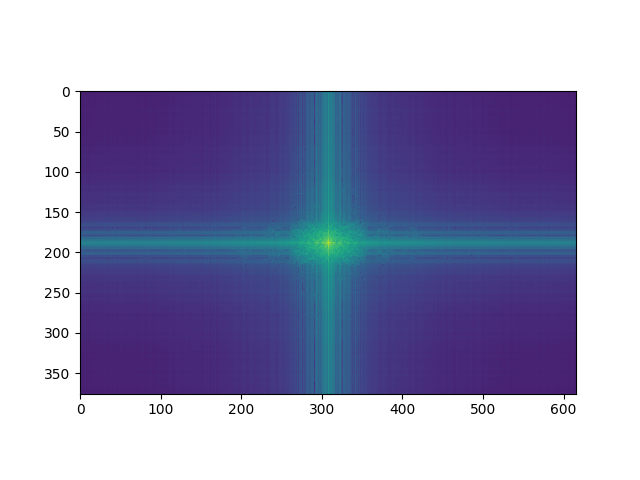 Lion After Low-Pass Filter
|
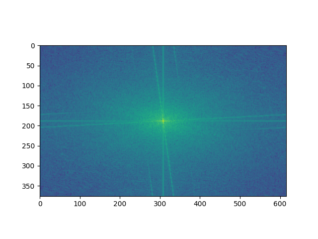 Cat Before High-Pass Filter
|
 Cat After High-Pass Filter
|
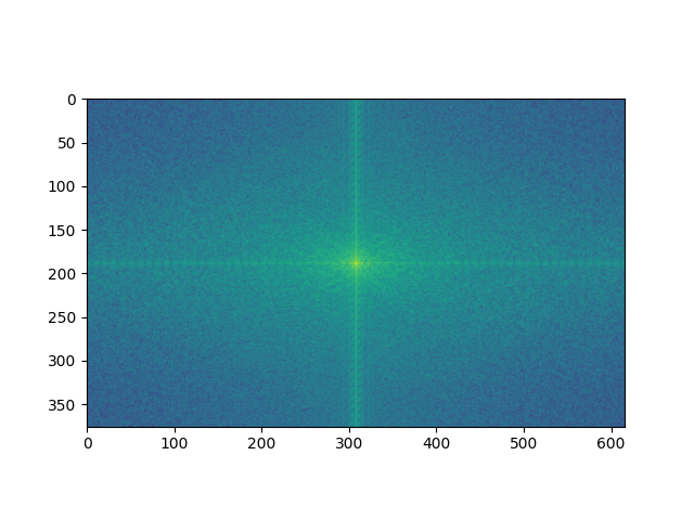
 Log Magnitude of the Hybrid Image
|
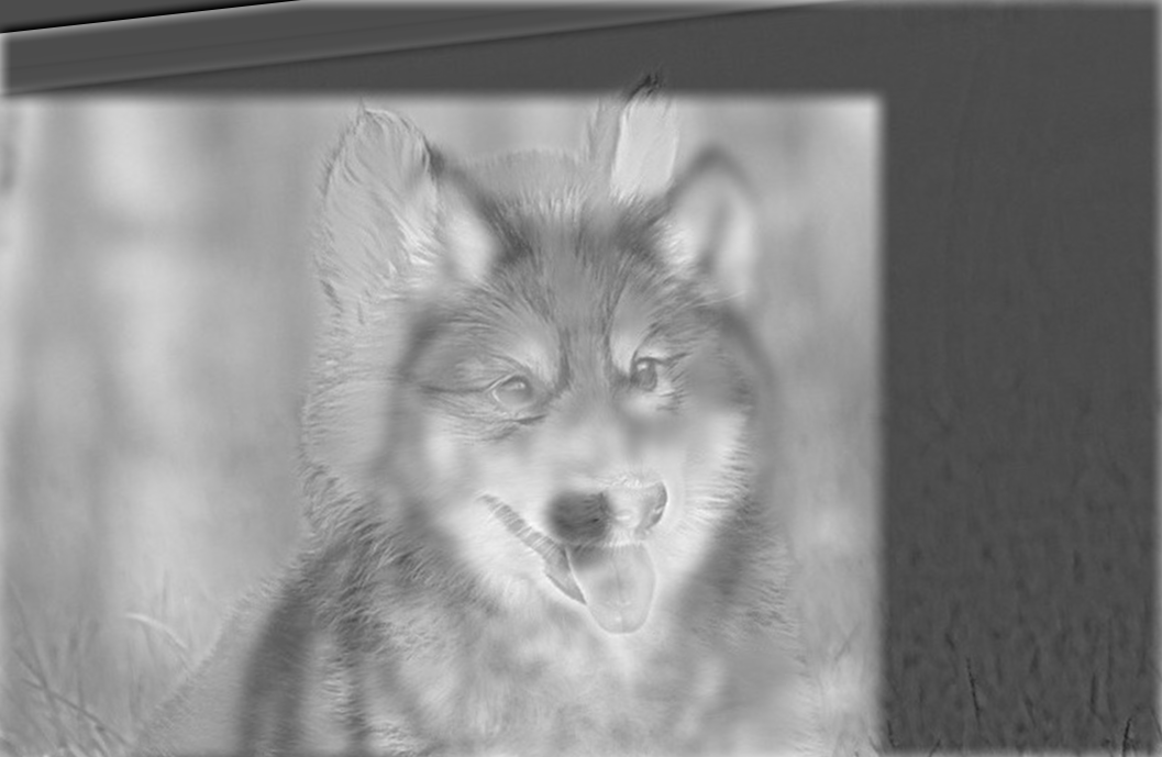
Failure Case:
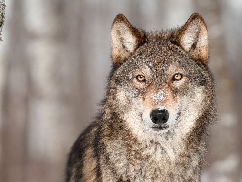 Wolf
Wolf
|
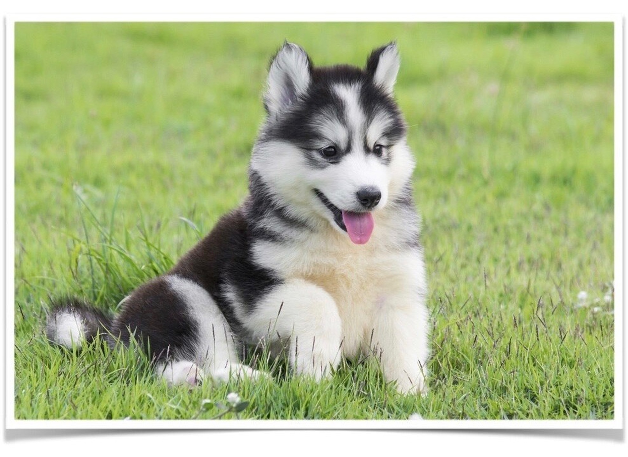 Husky
Husky
|
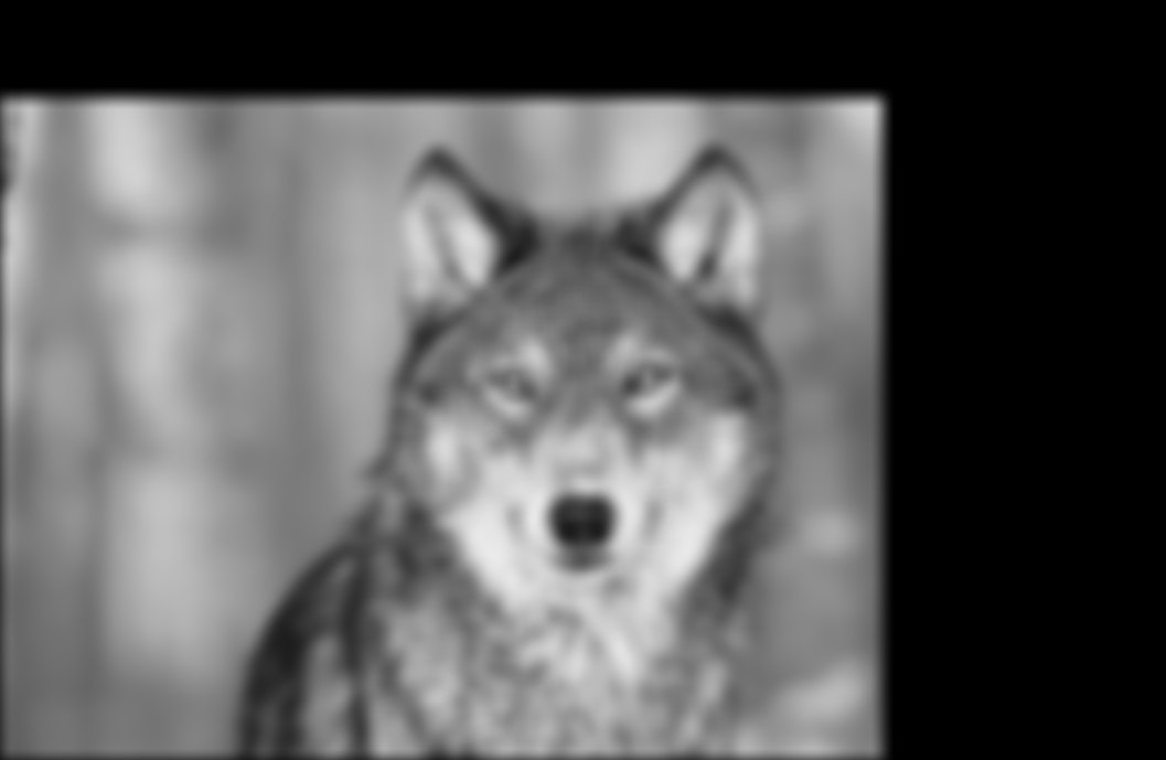 Low Frequency Image
(far away; Gaussian Blur applied)
|
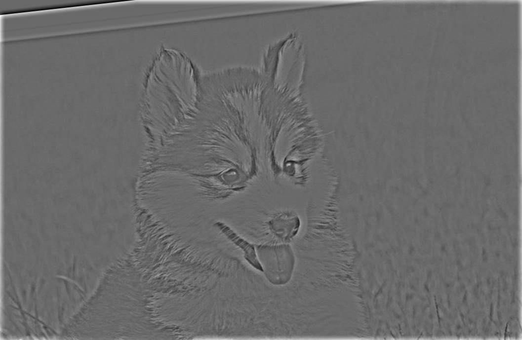 High Frequency Image (close up)
|
 Hybrid Image
|
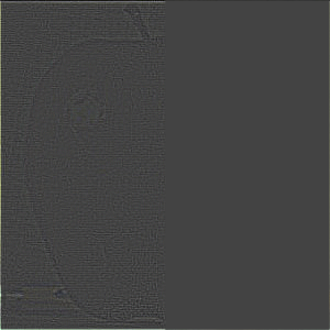
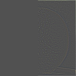
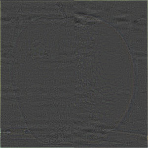
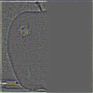
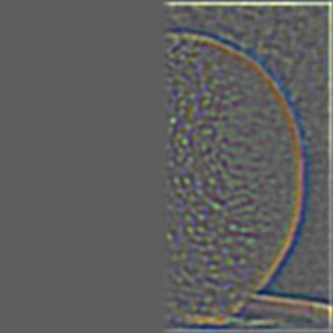
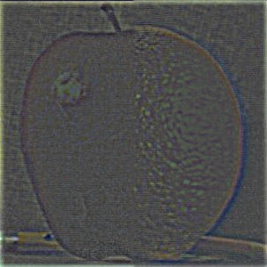
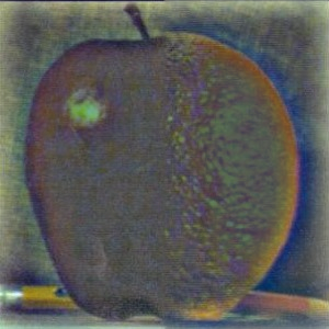
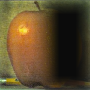
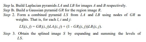
Section 2.3: Multi-resolution Blending and the Oraple journey - Gaussian and Laplacian Stacks
In this part of the project, we implement both a Gaussian and Laplacian stack. The former involves applying a Gaussian with larger and larger sigmas as we go down the stack, blurring the image more with each level. Using successive layers, we create a laplacian stack by taking the difference of two consecutive Gaussian stack layers. For constructing the Oraple, I used 7 layers. Here is my recreation of the outcomes of Figure 3.42 in Szelski page 167.
Section 2.4: Multi-resolution Blending
In this part of the project, we utilize both our Gaussian and Laplacian stack in order to implement multi-resolution blending for creating the oraple. The following is the general algorithm that we used for multi-resolution blending (except it utilizes pyramids instead of stacks, the former only additionally including downsampling for each level).
LionCat
 Blended LionCat
|
OskiBear
 Blended OskiBear
|
Bells & Whistles
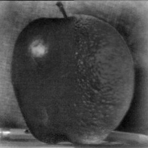 Black & White
|
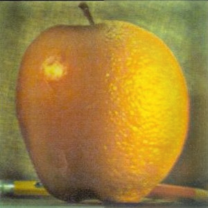 With Color
|
The coolest thing I learned about from this assignment was the vast use of gaussian kernels-- from being a low-pass filter to being able to smooth and blend images, and much more, this assignment made me really appreciate them and the power of their "simplicity" to create such complex and creative images.