CS194-26 Fall 2021 | Ryan Mei, cs194-26-aat

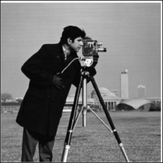
Part 1.1: Finite Difference Operator

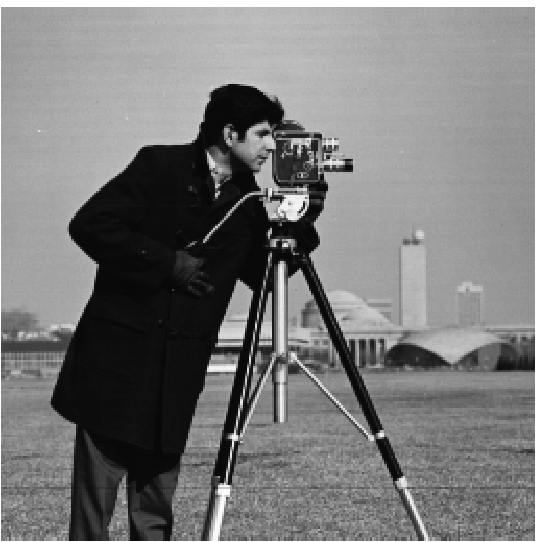
I first created a simple edge detector. To start we compute the the left-right and top-down gradients of the image using the simple kernels dx = [1, -2] and dy = [[1], [-1]]]].

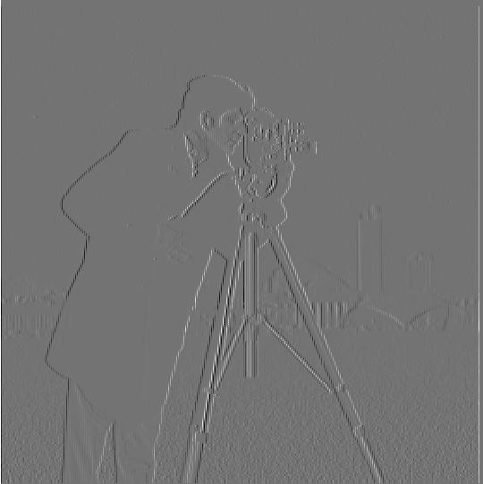
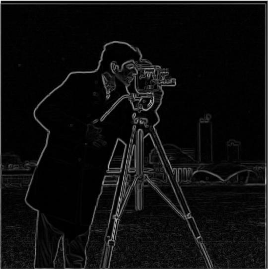
Using the horizontal and vertical gradients, the gradient magnitude is calculated by taking the root sum of squares of each pixel location in each gradient image.

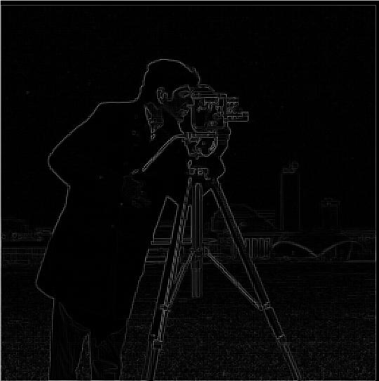
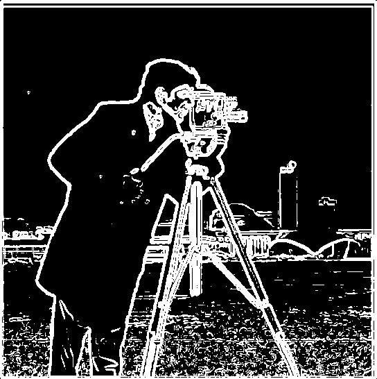
To create the edge-detected image, the gradient magnitude image is qualitatively thresholded then binarized.

Part 1.2: Derivative of Gaussian (DoG) Filter

Our naive edge detector amplifies all high-frequency data, regardless of whether it is a real edge or if it's just noise. Notice the tiny specks in the sky of the edge image above which remain even after setting a relatively strong threshold.

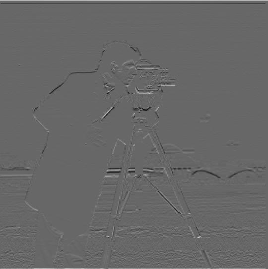
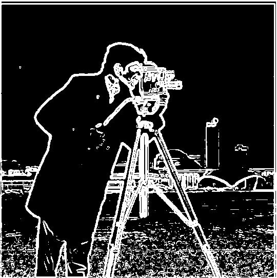
To resolve, this we can first low-pass filter our image by convolving it with a Gaussian kernel which reduces the shot noise.

We then take the horizontal and vertical gradients again, and calculate the gradient magnitude image.

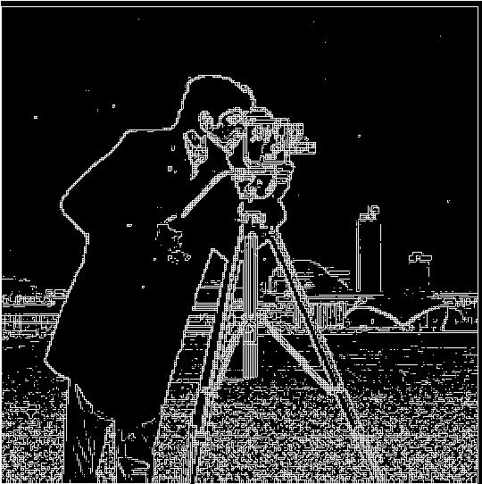
The gradient magnitude image is then thresholded and binarized to create a significantly less noisy edge image. Even though the thresholds are less than half than for the non low-pass filtered image, the edges are clearer and there is less noise. We can see that unfortunately this comes at the cost of our edges becoming thicker, since the edges are also high-frequency information.

We can also do this as a single convolution by convolving our horizontal and vertical difference kernals each with the Gaussian kernel. We verify that we get the same result:

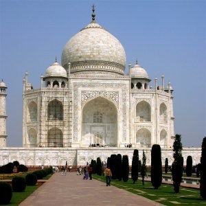
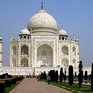
Part 2.1: Image "Sharpening"

The sharpening kernel used in this project is defined as (1+α)𝛿 - α*g where α is a positive constant, 𝛿 is the unit impulse, and g is a Gaussian kernel.

With a g with unit variance, and α=2, we can create a sharpened image of the Taj Mahal:

To test this sharpening kernel, we can test it on an image that we intentionally blur with a Gaussian kernel and compare it with the original.

Part 2.2: Hybrid Images (With Color!)

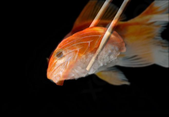
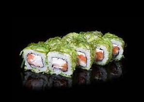
To fuse the contents of two images, we can high-pass filter one image and low-pass the other, then average the two. For example if we want to make a picture of goldfish nigiri to plan for what we're going to have for dinner:

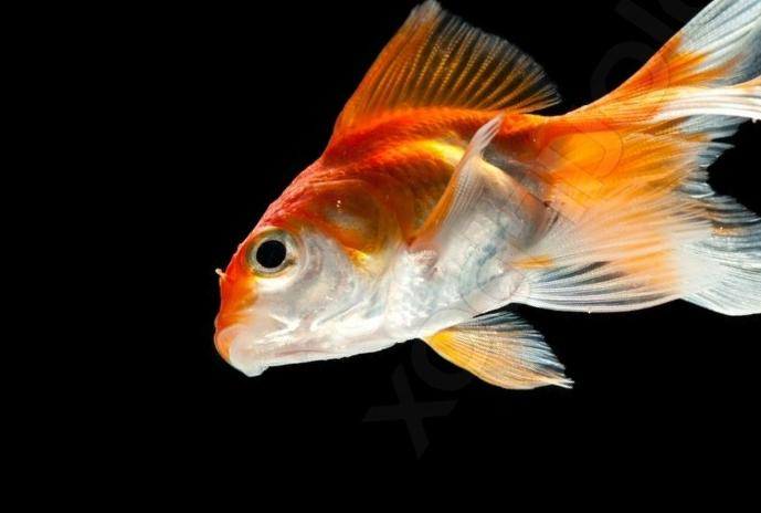
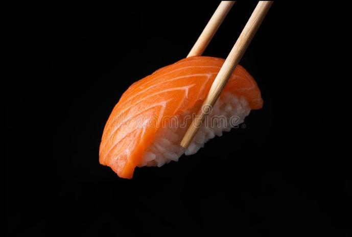
We still want to taste and feel the texture of the grains of our rice (as with all good nigiri) so we high pass filter the nigiri, and we want to feel the wriggling slimy body and fins of our goldfish but not necessarily the fine but rough scales so we low-pass filter our goldfish.

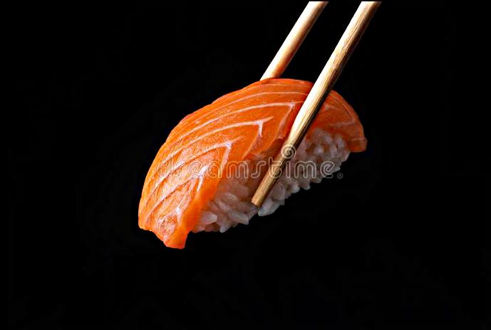
To create our supreme treat we average the pixels of the two images:

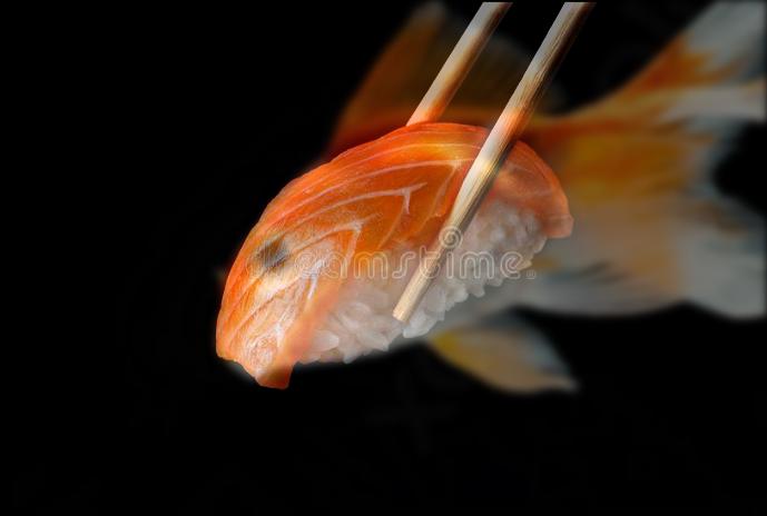
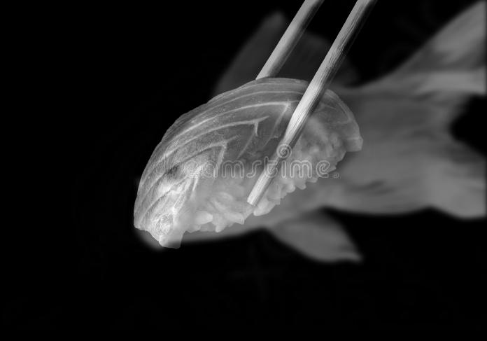
In our color implementation we use the color from both channels since we want the orange and white from both the nigiri and goldfish to blend seamlessly together. We can see that this looks a lot better than a simpler grayscale implementation:

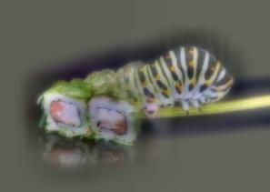
This method was also used to create some other delicious treats or mashups of people:

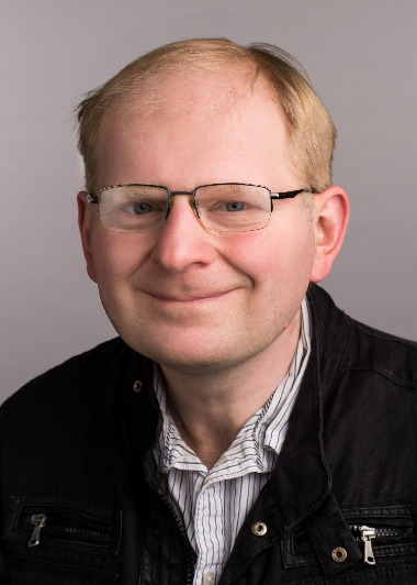
Failure analysis: We can see in the case of LincEfros, since their faces are not quite in the same orientation (Professor Efros is facing slightly toward the left) and since they have quite different face shapes, the resulting picture looks quite strange, kind of like it has two mouths and ears (one set blurry). This is accentuated by the fact that one image is color and the other is greyscale.

Part 3&4: Multi-resolution Blending (With color!)

To multi-resolution blend two images, we first create a Gaussian stack of each image by convolving each image with an increasingly wider Gaussian.

Next we subtract each lower-frequency image with the image with the next higher frequency information to create band-pass images, which make up our Laplacian stack.

We can do a sanity check that the sum our Laplacian stack gives us our original images (albeit with the colors slightly off).

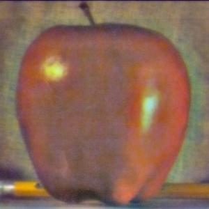
To actually blend the images together, we create a binary mask and a Gaussian stack of the mask. We use each layer of the Gaussian stack to weight the combination of our apple and orange images, with higher values meaning it draws more heavily on the apple pixel and lower values corresponding to more orange pixel.

We multiply each mask in place with the corresponding apple/orange orange Laplacian layer, then sum all the images together to create our final blended Orapple!

Though the colors are slightly off, it still looks significantly more delicious than the same procedure with only greyscale inputs!

We can make more delicious snacks using our multi-resolution blending algorithm!

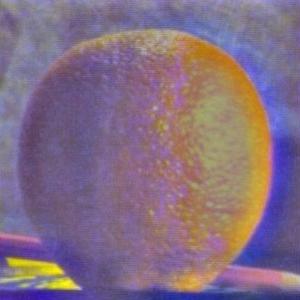
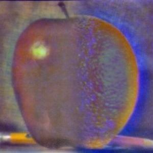
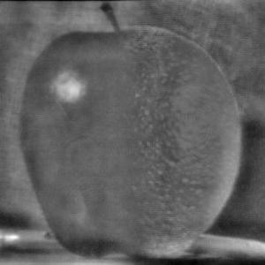
We can also take a Gaussian stack of an irregularly shaped mask, like a circle.

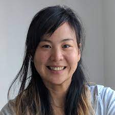
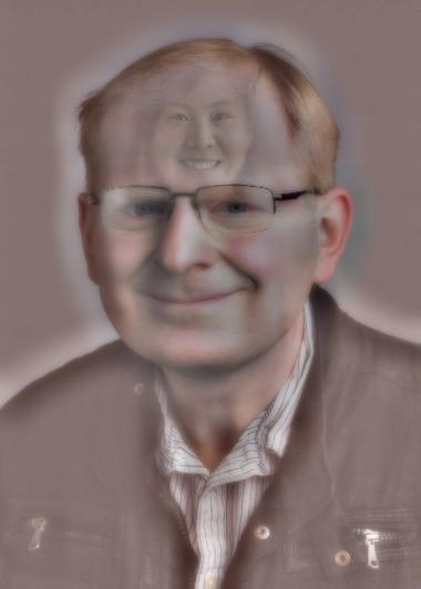
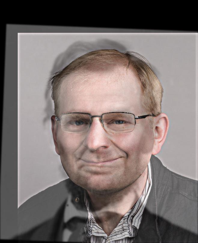
We can use this to give Professor Efros new and exciting powers like (hopefully eventually) Professor Kanazawa's great hair! Whoops that didn't quite work did it, but at least we have Efroszawa!