Fun with Filters and Frequencies

Introduction

Convolution with filters has a wide application in computational photography. Image blurring, sharpening and blending all depend on this fundamental operation. Moreover, popular convolutional filters (such as Gaussian filters) can also achieve amazing effects: blending high and low frequencies together can result in an image that looks differently from near and far away. In this project, we will discover all the above applications of image filters, and visualize their results.

Image Derivatives

In this part we will explore how to use convolution to find derivatives of an image. Recall that in a continuous case, $\frac{df}{dx}=\underset{\mathrm{\Delta }\to 0}{lim}\frac{f(x+\mathrm{\Delta })-f(x)}{\mathrm{\Delta }}$$\frac{df}{dx} = \lim \limits_{\Delta \rightarrow 0} \frac{f(x + \Delta) - f(x)}{\Delta}$. However, since images are represented in discrete form, we will apply the approximate representation of derivatives while dealing with images. Namely, for the $x$$x$ derivative, $\frac{\partial I(x,y)}{\partial x}=I(x+1,y)-I(x,y)$$\frac{\partial I(x, y)}{\partial x} = I(x + 1, y) - I(x, y)$. For the $y$$y$ derivative, $\frac{\partial I(x,y)}{\partial y}=I(x,y+1)-I(x,y)$$\frac{\partial I(x, y)}{\partial y} = I(x, y + 1) - I(x, y)$. Written in a convolutional form, computing the $x$$x$ derivative of an image is the same as convolving the original image with $\left[\begin{array}{cc}1& -1\end{array}\right]$$\begin{bmatrix}1 & -1\end{bmatrix}$, and computing the $y$$y$ derivative of an image is the same as convolving the original image with $\left[\begin{array}{c}1\\ -1\end{array}\right]$$\begin{bmatrix}1\\-1\end{bmatrix}$.

Now we will experiment image partial derivative with cameraman.png.

Here is the visualization of $x$$x$ derivative and $y$$y$ derivative:

$x$$x$ derivative:

$y$$y$ derivative:

Now we apply Gaussian blur to the original image. I used Gaussian kernel with size = 3 and $\sigma$$\sigma$ = 0.8. The resulting blurred version is as follows:

If we calculate the $x$$x$ derivative and $y$$y$ derivative of the blurred image, we can see that the derivatives are decreased (or softened) as well:

$x$$x$ derivative:

$y$$y$ derivative:

Another way to calculate the partial derivatives of the blurred image is to first convolve Gaussian filter with $\left[\begin{array}{cc}1& -1\end{array}\right]$$\begin{bmatrix}1 & -1\end{bmatrix}$ and $\left[\begin{array}{c}1\\ -1\end{array}\right]$$\begin{bmatrix}1 \\ -1\end{bmatrix}$, and then apply the resulting filter to the original image. Since convolution obeys the communicative law and associative law, the final results should be the same:

$x$$x$ derivative:

$y$$y$ derivative:

Image Sharpening

Another image manipulation we can do with convolution is image sharpening. To do sharpening, we first apply Gaussian blur to the original image to extract its low frequencies. We then extract the low-frequency image from the original image to get high frequency portions. The obtained high frequency portion is then added to the original image by some specified weight. The higher the weight of the high frequency portion, the shaper the resulting image will be.

Below is the original image and sharpened version of taj.jpeg:

Original image:

Sharpened version:

Here are two more examples of the effect of unsharp filter. The first image: big_sur.jpeg contains a low-resolution photo. We can see that after applying the unsharp filter, the photo looks sharper, and clearer due to additional high frequency.

Original image:

Sharpened version:

The final set of images contains three components: the original image, rainbow.jpeg, the blurred version, and the sharpend version after blurring the image.

Original image:

Blurred version:

Sharpened version:

Image Hybrid

From now on we will explore some amazing things about convolution filters. The first one is image hybrid. In particular, image hybrid is putting two pictures of different frequencies together, such that viewers can see the high-frequency image from near, and low-frequency image from far away.

To achieve this effect, we will first pick two images, and pick two points on both of them to indicate where they should be aligned together. After that, we will pick one image $A$$A$ to retain its high resolution portion, and the other image $B$$B$ to retain its low resolution portion. We stack these two images together (add them up) with specified weight to obtain the new hybrid image. When we look at this hybrid image closely, we can see image $A$$A$, which dominates the high-frequency portion, and as we see the image from afar, we can see image $B$$B$, which dominates the low-frequency portion.

Below is our first example: to hybrid DerekPicture.jpg with nutmeg.jpg. Looking closely, the viewer should see the cat, and backing afar, the viewer should see Derek.

Here are two more examples of my choice. The first is hybriding two people together, while the second is hybriding two animals.

Original Image 1:

Original Image 2:

Alexei Kanazawa

Original Image 1:

Original Image 2:

Lion Wolf

Looking at the three hybrid images above, we may see that the hybrid effect is the worst when we blend two faces together. This is probably due to the fact that facial features differ significantly between individuals. Therefore, it is hard to align two faces perfectly, so we could still somehow see the other image wherever we stand. Moreover, we have one original image to be black-and-white, and another is colored. By forcing both images to be black-and-white, we may lose some information in the colored image.

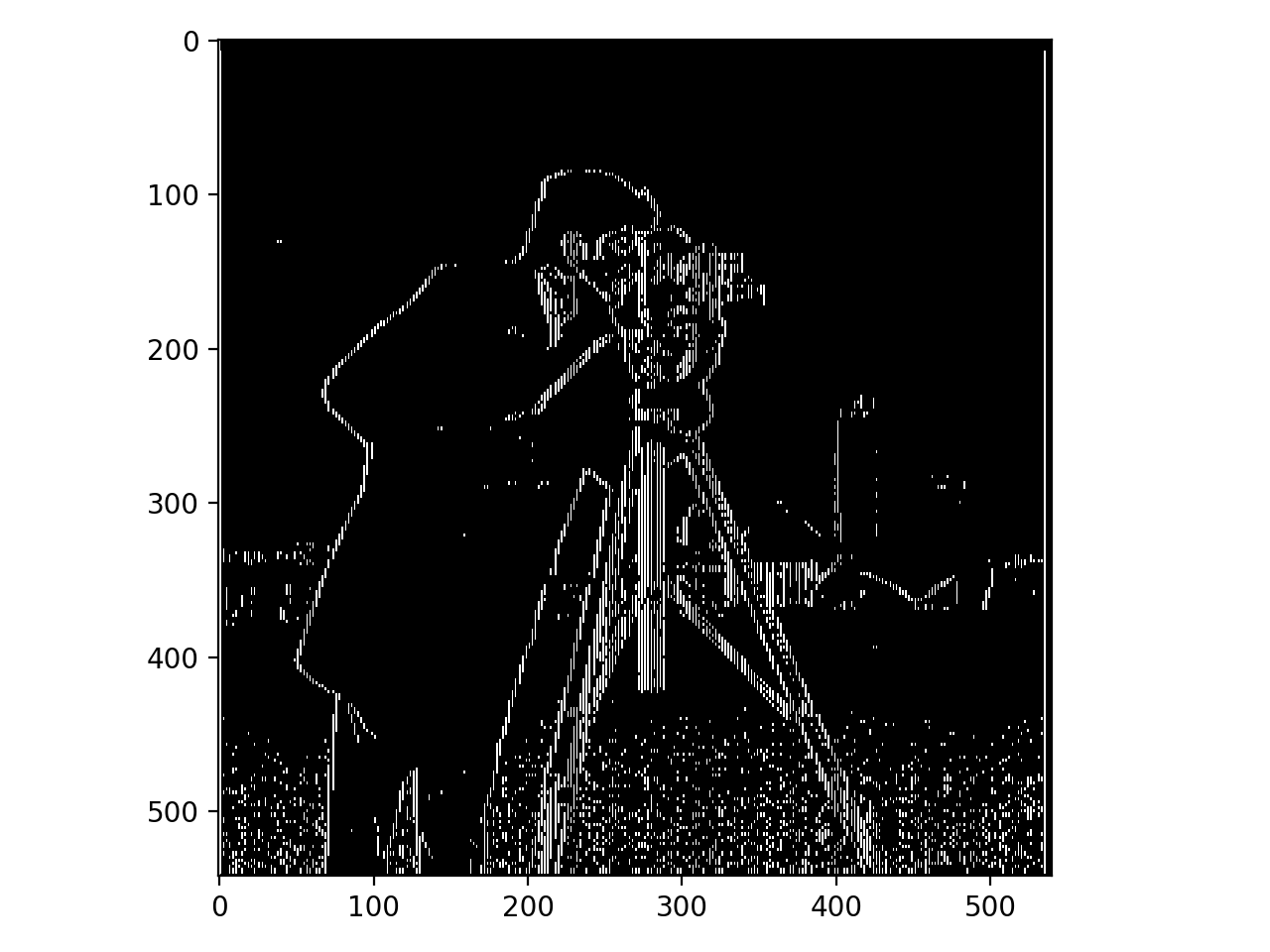
To analyze how hybrid convolution works, we will visualize the images through Fourier transform, and see how high-pass and low-pass filters manipulate frequencies of the images. The below visualization is based on wolf-lion hybrid. In the images below, points farther away from the center represent higher frequency, while the brightness of a point represents the magnitude of that frequency.

We can see that while passing an image through a Gaussian kernel, most high-frequency points are filtered out. In contrast, if we pass the image through a high-pass filter, the resulting image would emphasize those high-frequency points, and weaken the low-frequency points. Combining low-frequency and high-frequency images, we can get a hybrid image that covers all frequencies.

Lion Original Frequency

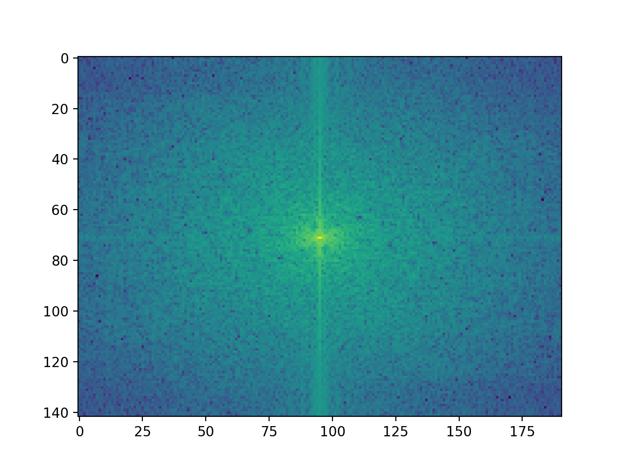
Wolf Original Frequency

Wolf Low Frequency

Lion High Frequency

Combined Frequency

We can also try hybriding two colored images together. What I did was to apply filtering and addition on each of the R, G and B channels, and then stack the results together. Here is the resulting image of hybriding DerekPicture.jpg and nutmeg.jpg :

It seems from the image that it works better to use color for the low-frequency component. This is probably because color tend to appear in patches. However, a high-pass filter would filter out low-frequencies (where colors may lie), leaving only strengthened outline of objects. Therefore, images tend to be less colorful after being passed though a high-pass filter.

Guassian and Laplacian Stacks

In this part we are creating multi-resolution images using Gaussian and Laplacian stacks. The idea is taken from Burt and Adelson's paper in 1983: "A Multiresolution Spline With Application to Image Mosaics". Different from the original implementation, we are not downsampling/ upsampling the images at each level. Rather, we are only expanding the size of kernel each time to achieve the same multi-resolution effect.

To implement Gaussian stack, we apply Gaussian kernel on the original image multiple times, each level with a greater kernel, resulting in images of lower resolution. The Laplacian stack is obtained by subtracting image at the next (lower) resolution level from the image at the current resolution level.

The results of a Gaussian stack should be a series of images with lower and lower resolution, while those of a Laplacian stack should be increasingly blurry outlines of objects in the image.

Here are the second, fourth and sixth level of Gaussian stack, applied to oraple.jpeg. For full series of images, please click here:

Gaussian stack Lv.2:

Gaussian stack Lv.4:

Gaussian stack Lv.6:

Here are the second, fourth and sixth level of Laplacian stack, applied to oraple.jpeg:

Laplacian stack Lv.2:

Laplacian stack Lv.4:

Laplacian stack Lv.6:

Image Blending

In this final part, we are going to explore an interesting application of Gaussian filters and Laplacian filters. In particular, we will try to blend two images together, such that they look like one whole picture.

In order to achieve this effect, we will blend the two images on multiple scales. To start with, we apply Laplacian stack to the two images to extract features at multiple resolutions. Then we devise a mask that indicates the way we want to blend the two images. The mask is then passed into a Gaussian stack to be blurred multiple times. Each level of the Gaussian blur corresponds to each level of the Laplacian stack. Finally, we iterate through the Laplacian stack of two images, and at each level, we combine the two images with a Gaussian-blurred mask. The final combined Laplacian stack is then added to get the result.

I experimented this strategy with four images. The first two images are from apple.jpeg and orange,jpeg. I tried on both gray-scale version and colored version.

Original Apple:

Original Orange:

Blended Gray Oraple:

Blended Color Oraple:

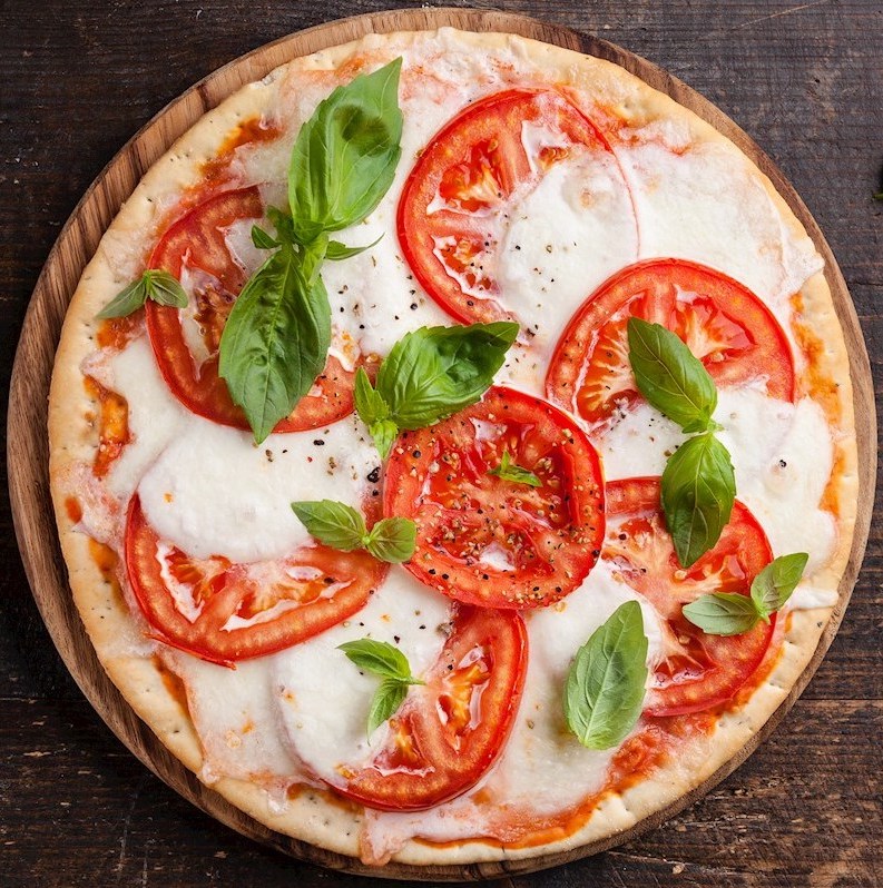
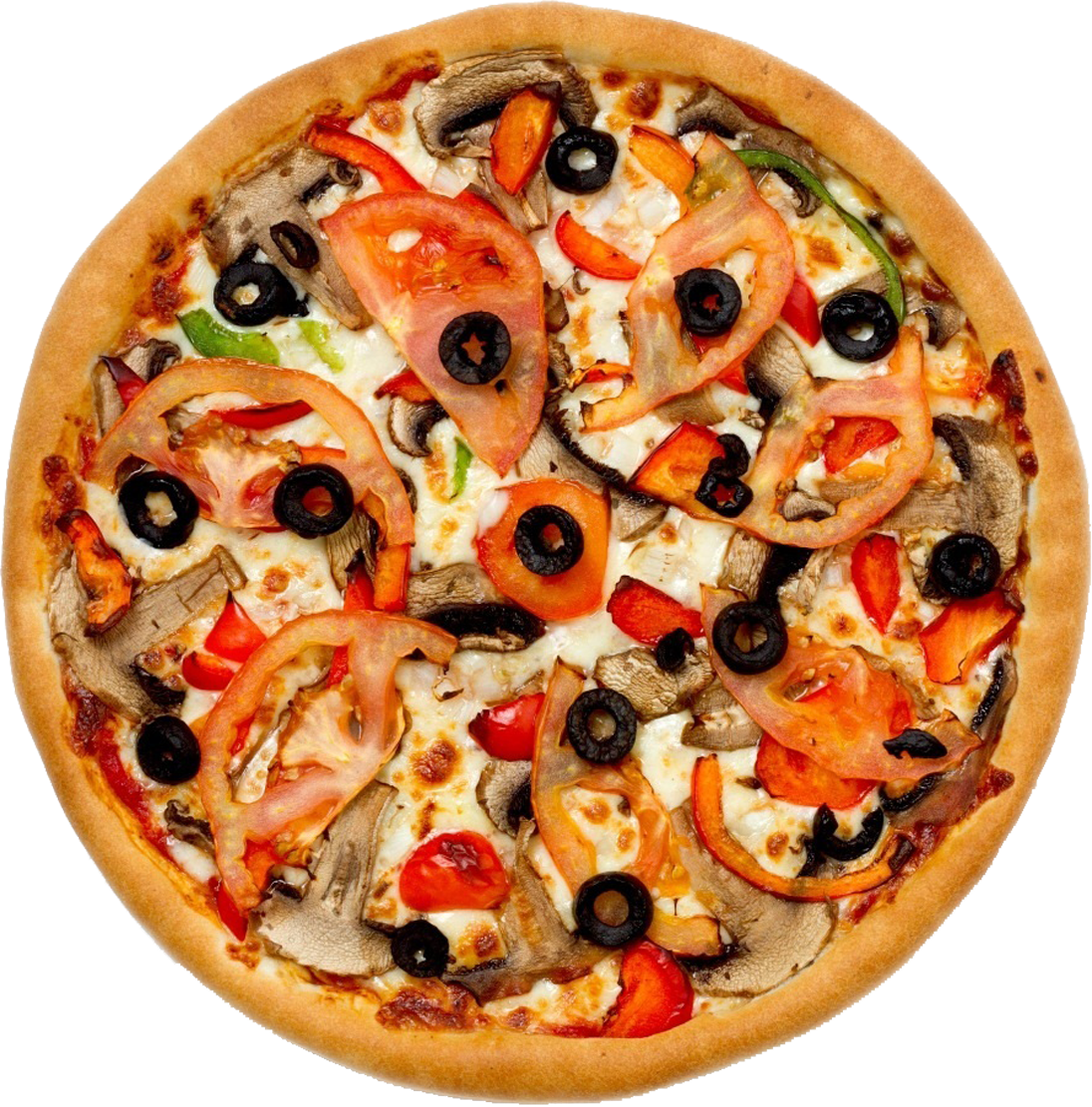
I then selected two images of different pizza, and blended them together in the colored version.

Original Pizza 1:

Original Pizza 2:

Blended Pizza:

Finally, here's the blended image of two squirrels using irregular mask:

Original Squirrel 1:

Original Squirrel 2:

Blended Squirrel:

The mask used by this blending is shown below: