Fun with Filters and Frequencies!

Part 1.1: Finite Difference Operator

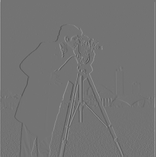
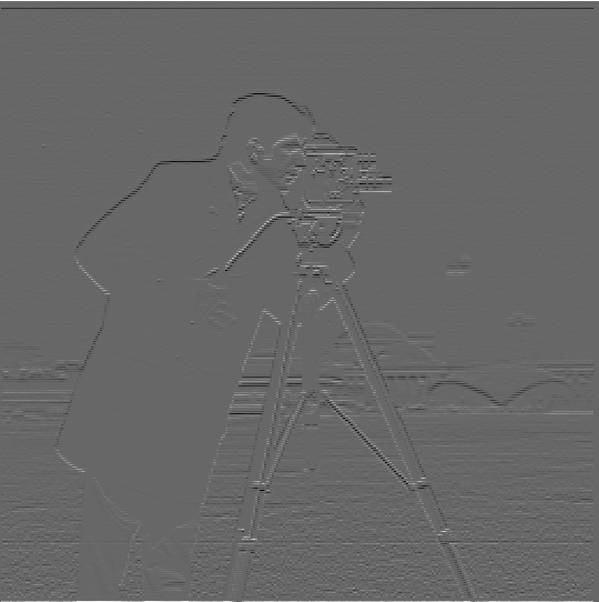
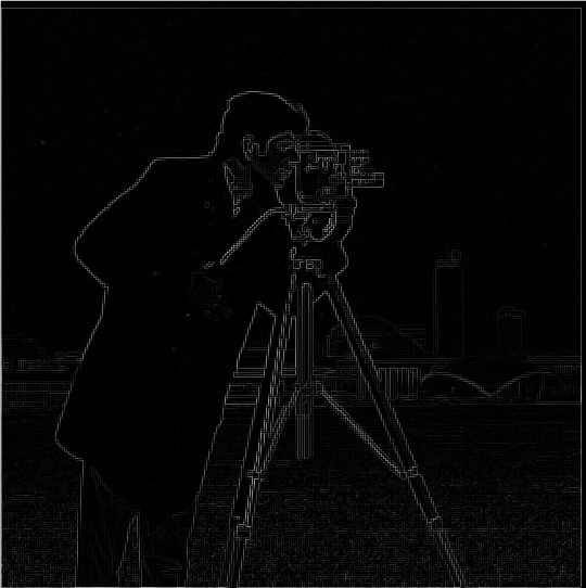
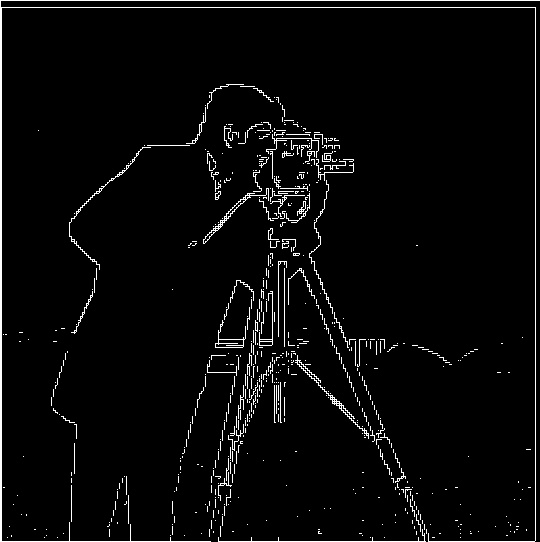
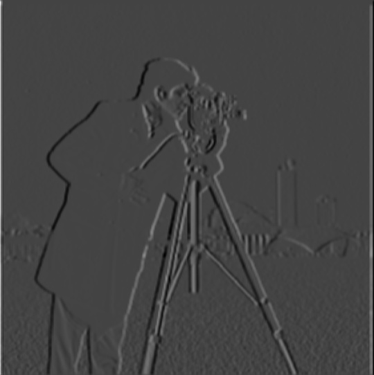
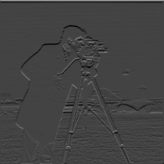
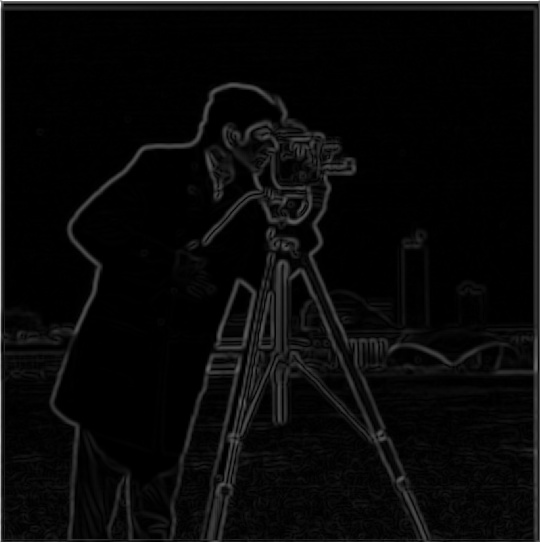
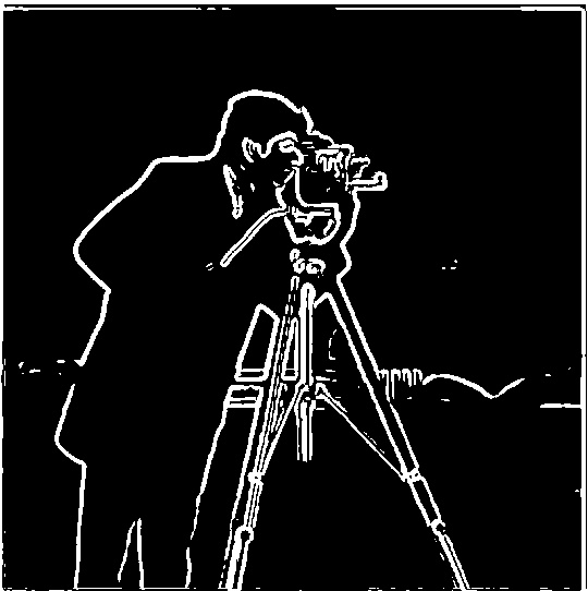
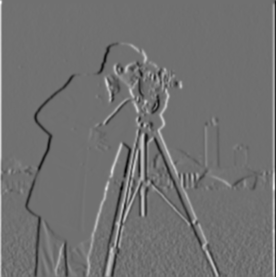
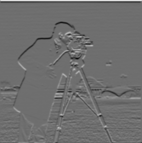
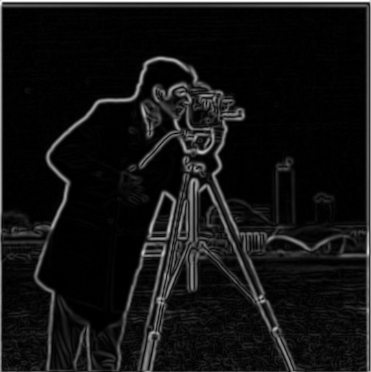
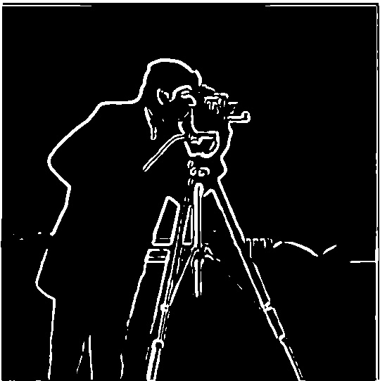
For this part, I found the partial derivative in both x and y of the cameraman image. Then to compute the gradient magnitude image, I squared these two resultant images that were convolved with Dx and Dy, summed them together, and took the square root. Then, I thresholded the image with 0.25. This means that pixels greater than this threshold were set to 1, else set to 0.

Here are the images of the cameraman convolved with Dx and Dy, respectively. Below those two images are the gradient magnitude image before thresholding, and then shown after thresholding.

Part 1.2: Derivative of Gaussian (DoG) Filter

First, I blurred the image with a Gaussian Kernel (with parameters ksize=16 and sigma=2). Then after blurring, I perform the above operations, convolving with Dx and Dy, then find the gradient image before thresholding the image as well. For this part, I used 0.065 as the new threshold value.

Below, I present the images of the cameraman in the same order as was presented above.

The differences I find in this method are that blurring the image with a Gaussian kernel before finding the gradient magnitude image results in much better defined and clearer edges.

The second method tried in this section incorporates everything into a single convolution by taking derivatives of Gaussian filters. These are known as the Derivative of Gaussian (DoG) filters, and are presented below. The gaussian kernel that we use is the same as above. The following images are then the cameraman convolved with the DoG filter on Dx and the DoG filter on Dy, from which the gradient magnitude image is found again.

As seen, this DoG method again produces the same stellar results!

Part 2.1: Image "Sharpening"

To sharpen images, my methodology is as follows. First, I blur the image with a Gaussian Filter and subtract that blurred image from the original image. We denote this difference as the high frequency version of the image. Then, we amplify this high frequency version by a value alpha and add it back to the original image, resulting in a sharpened image.

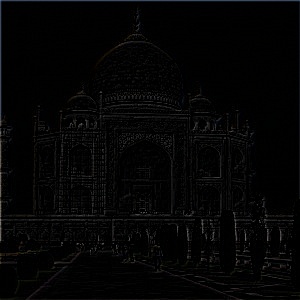
Below, I show my results performed on the Taj Mahal, and then on Cerulean City. I show the original image, blurred version, high frequency image, and then sharpened image, in that order. For both images, I use a Gaussian Kernel with ksize=4, sigma=1, and alpha=2.

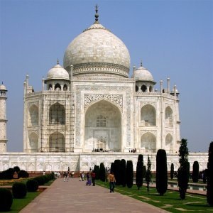
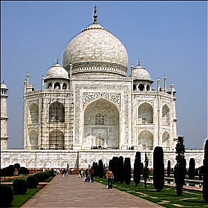
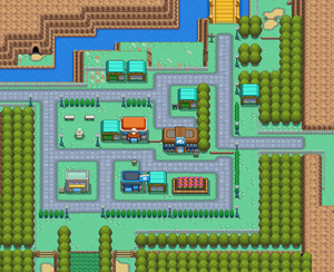
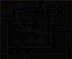
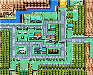
The sharpened Taj Mahal looks very nice. However, the sharpened Cerulean City looks a little offputting. Perhaps this is due to the fact that the original image is generated for a video game and has already been processed to look "optimal" for viewers.

Part 2.2: Hybrid Images

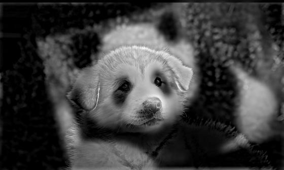
Here, I show some hybrid images that I've generated. To do so, I low-pass filter one image and high-pass the other image, before aligning and adding the two to create the hybrid image. For all of the below, I use a high filter sigma of 10000 and a low filter sigma of 300. For both of these kernels, ksize = 15.

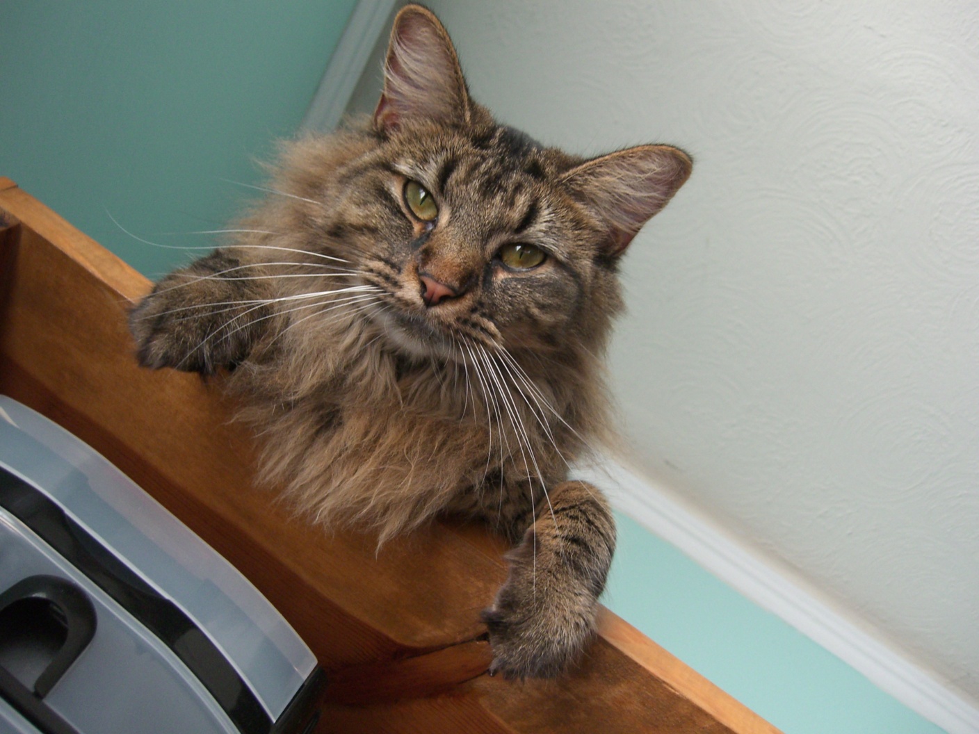
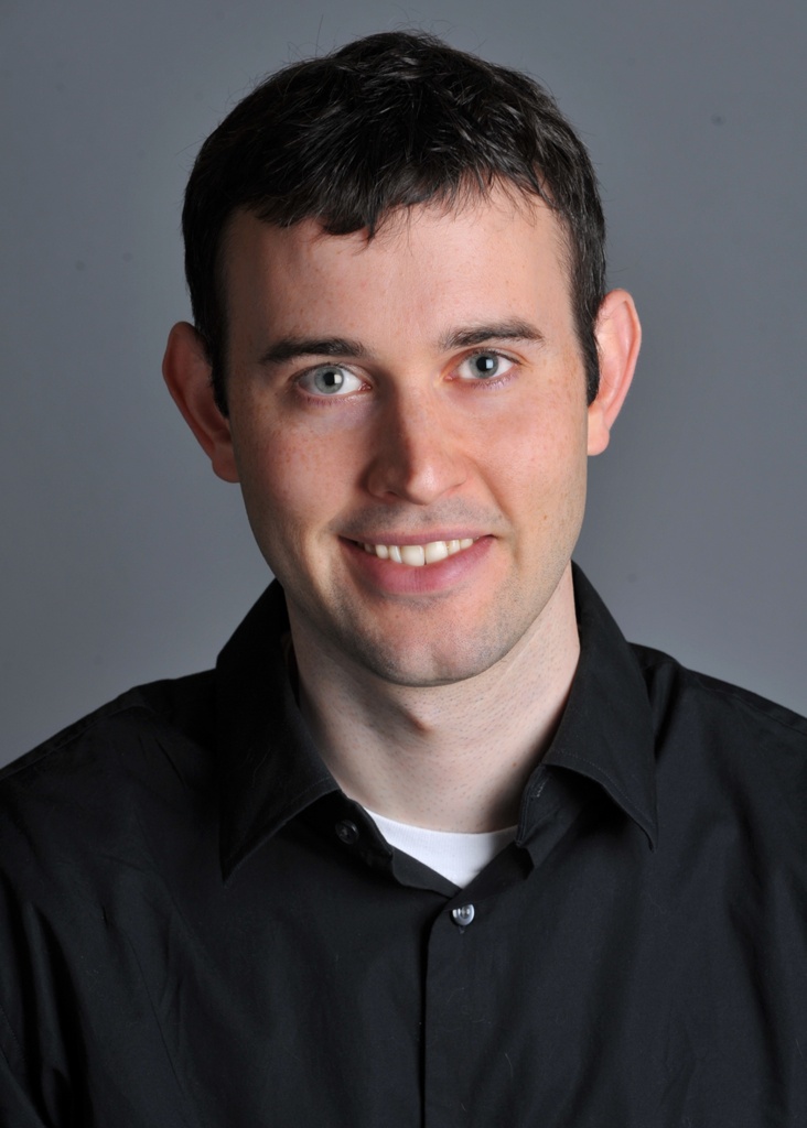
My first example is hybridizing Nutmeg and Derek.

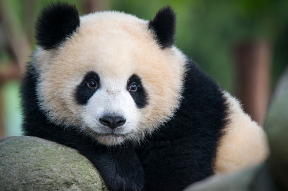
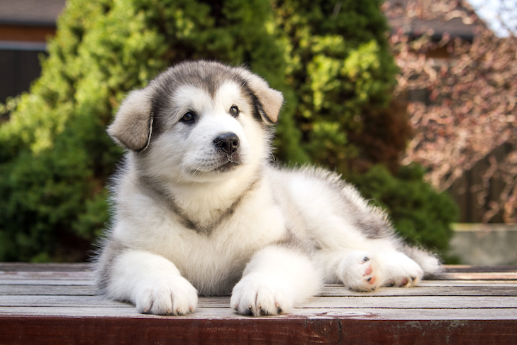
My second example is hybridizing a panda and a puppy.

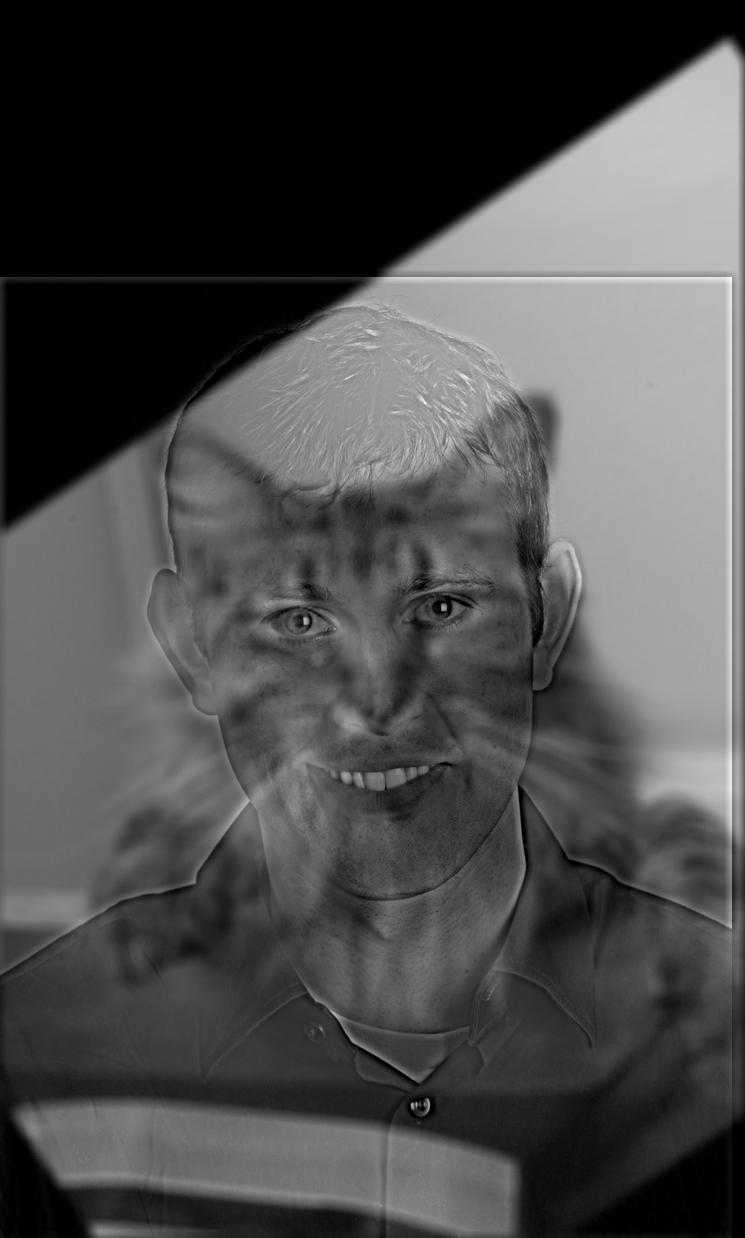
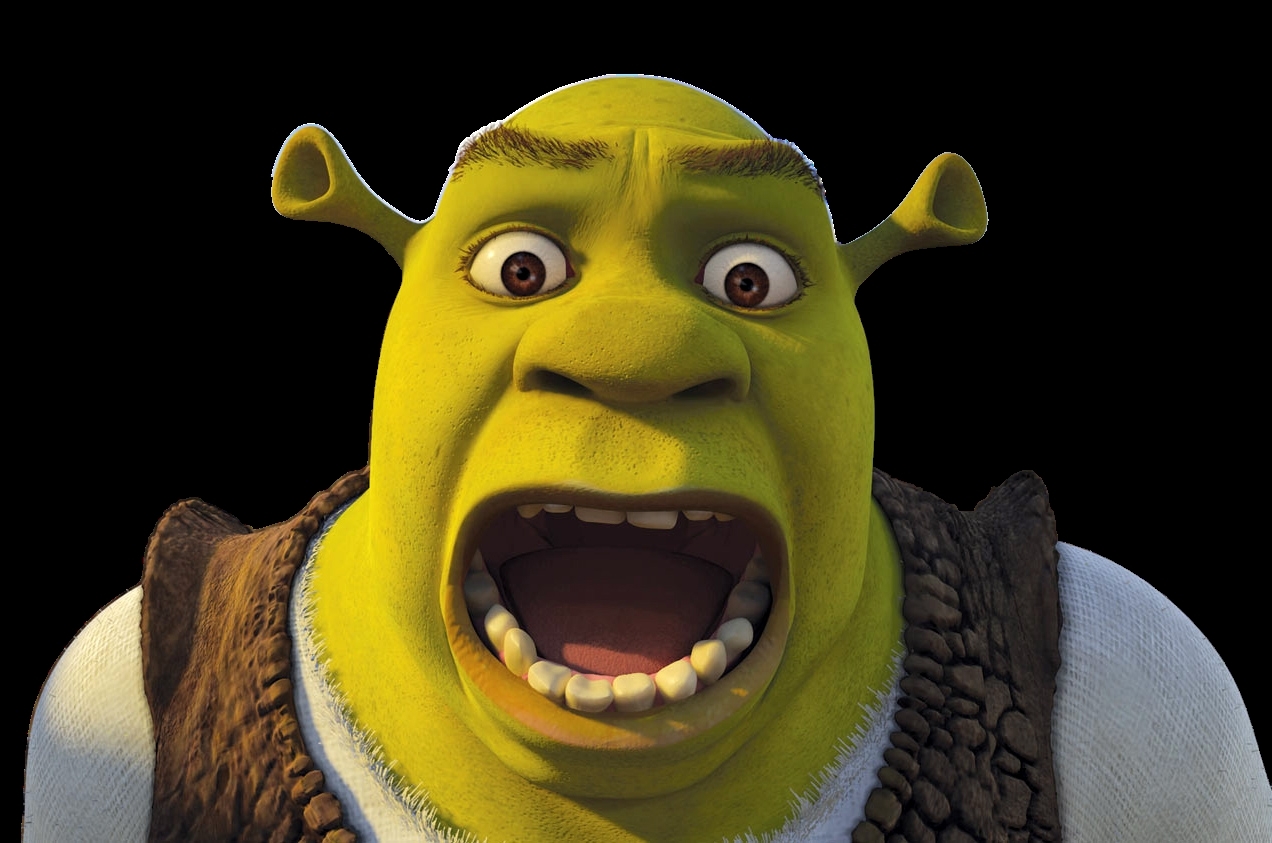
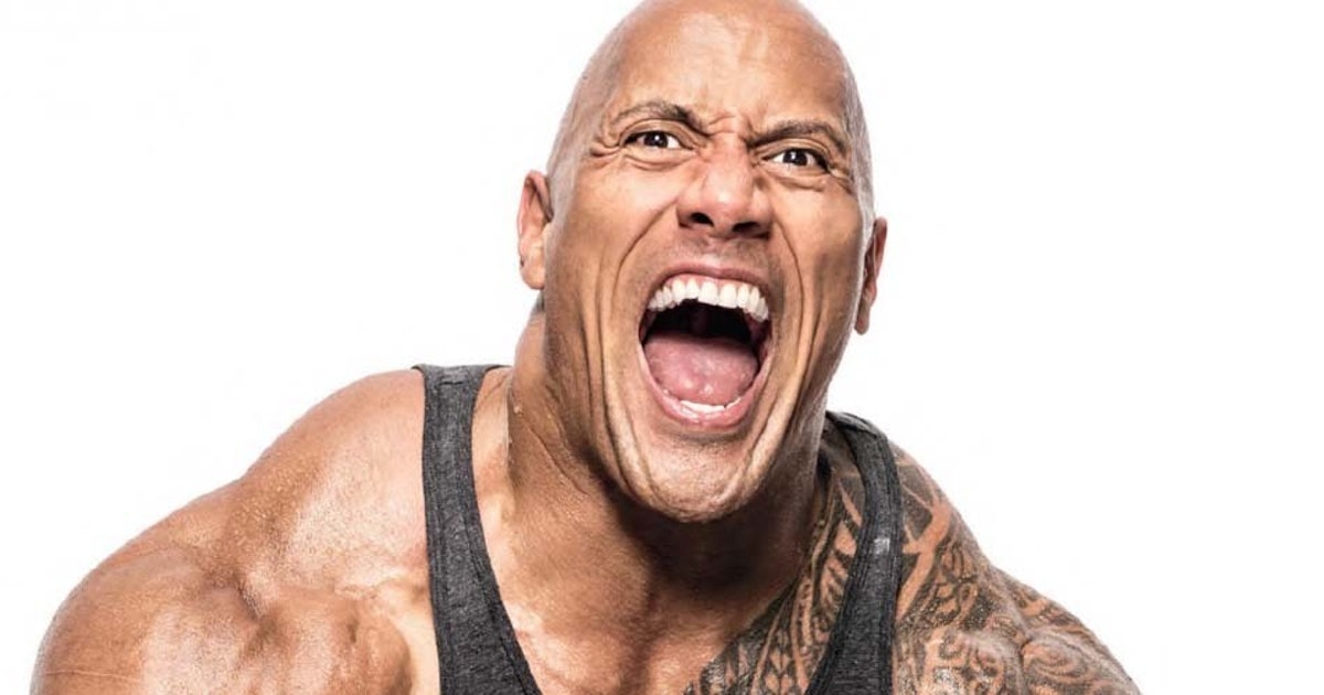
My third example is hybridizing Shrek and The Rock. I really enjoyed this effect, so I switched around the ordering of the images to see how both looked.

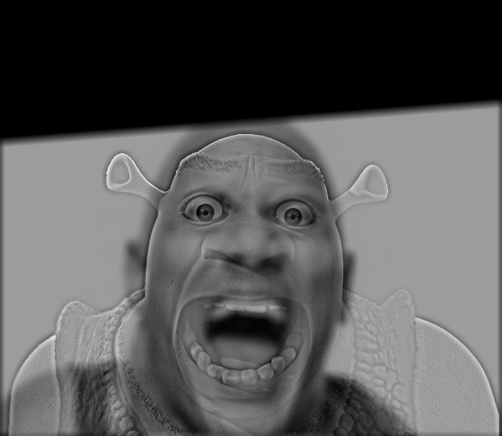
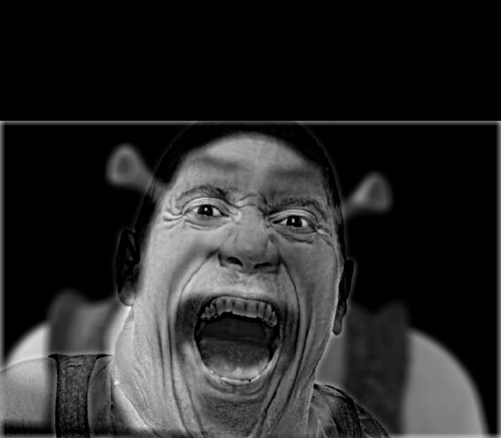
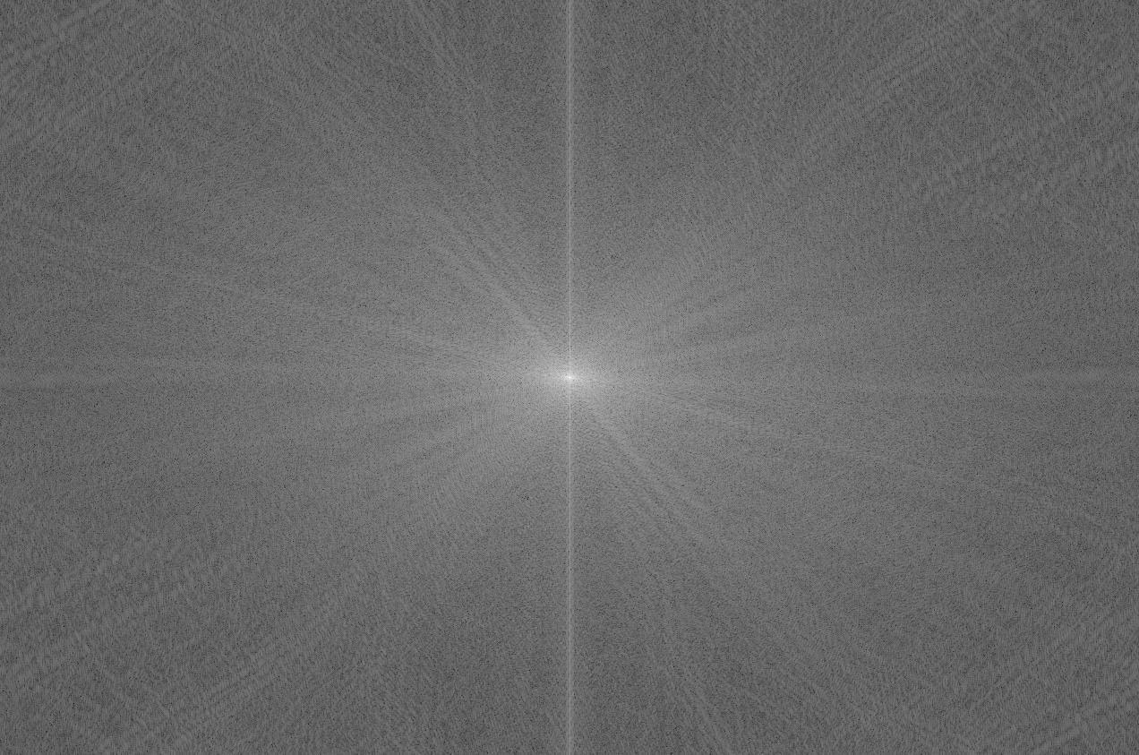
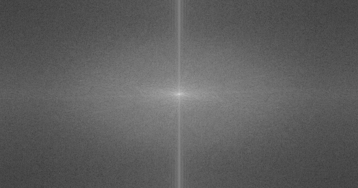
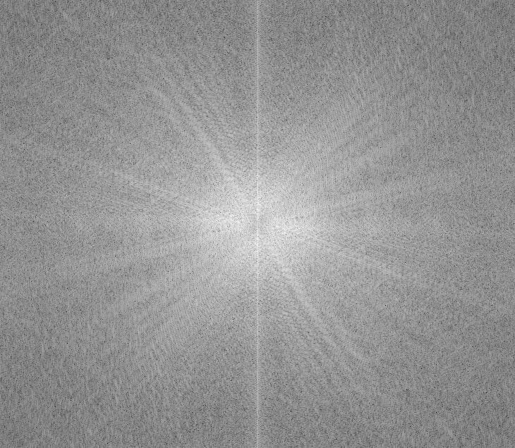
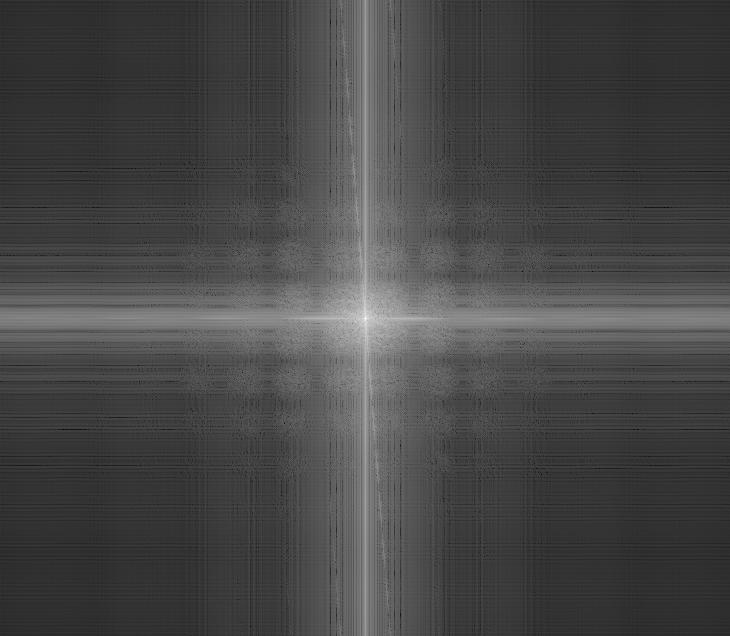
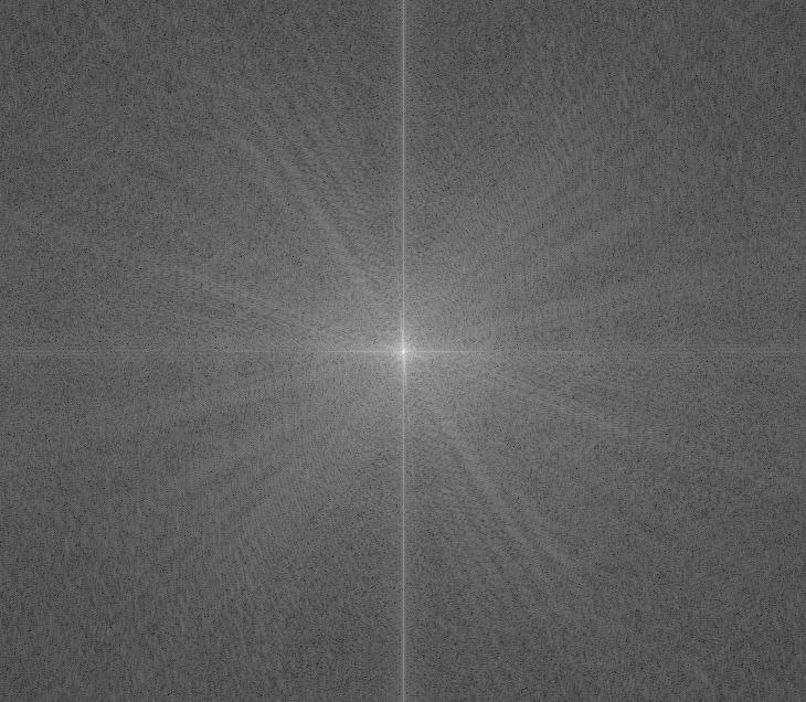
For this example, I'll also show the process through frequency analysis. Below, the log magnitude of the Fourier transforms of the input images, the high and low filtered images, and the hybrid image are shown (in that order).

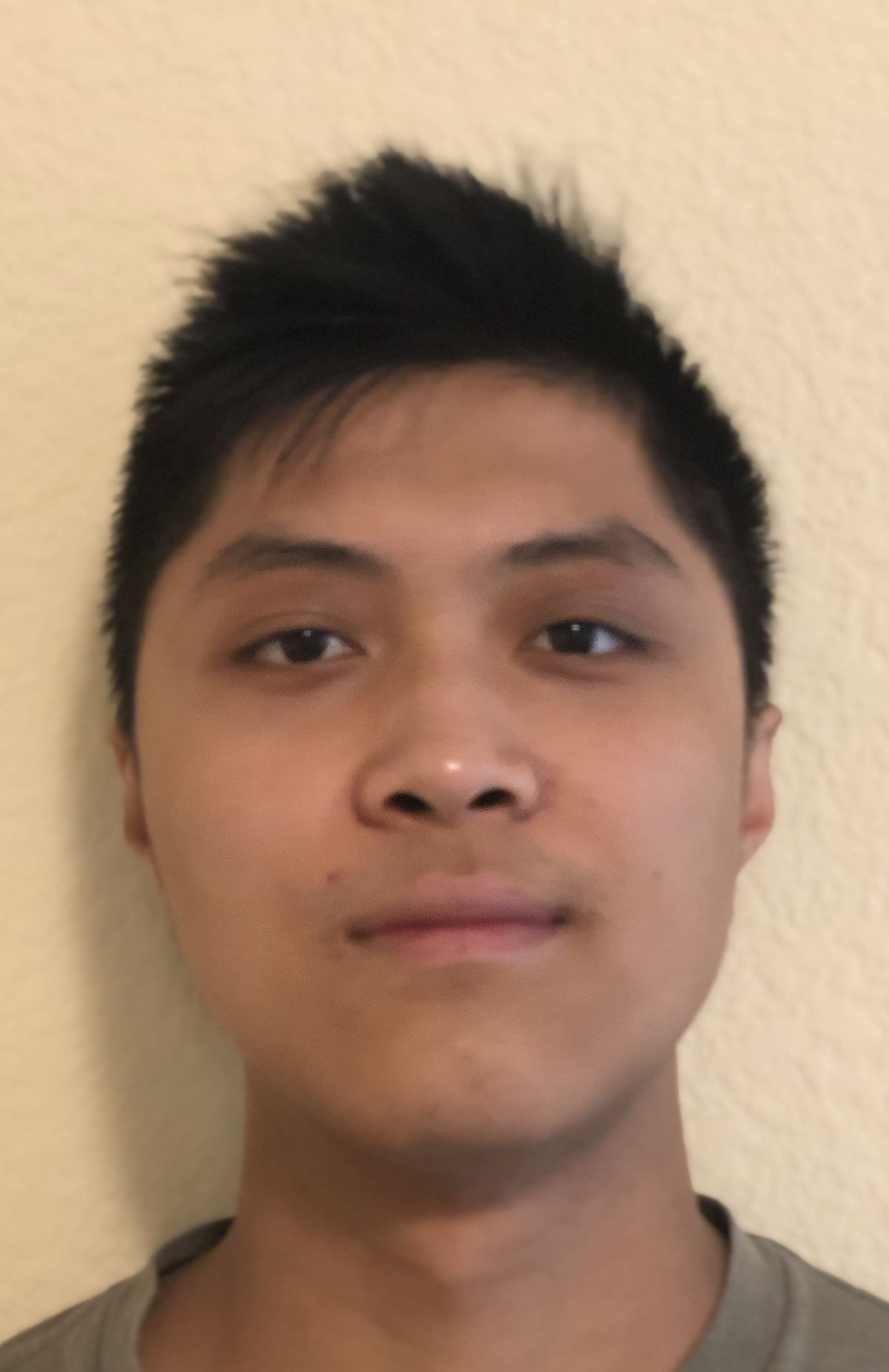
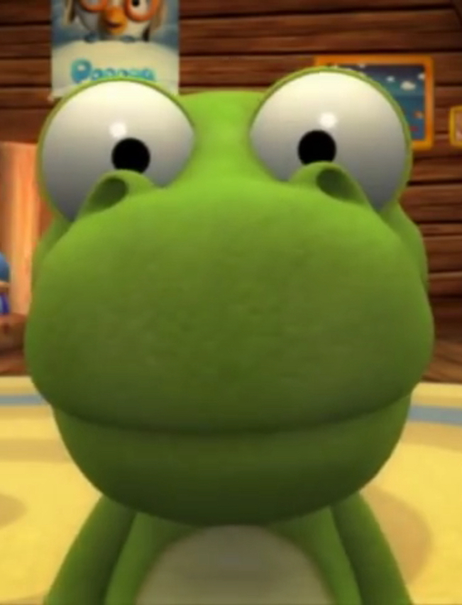
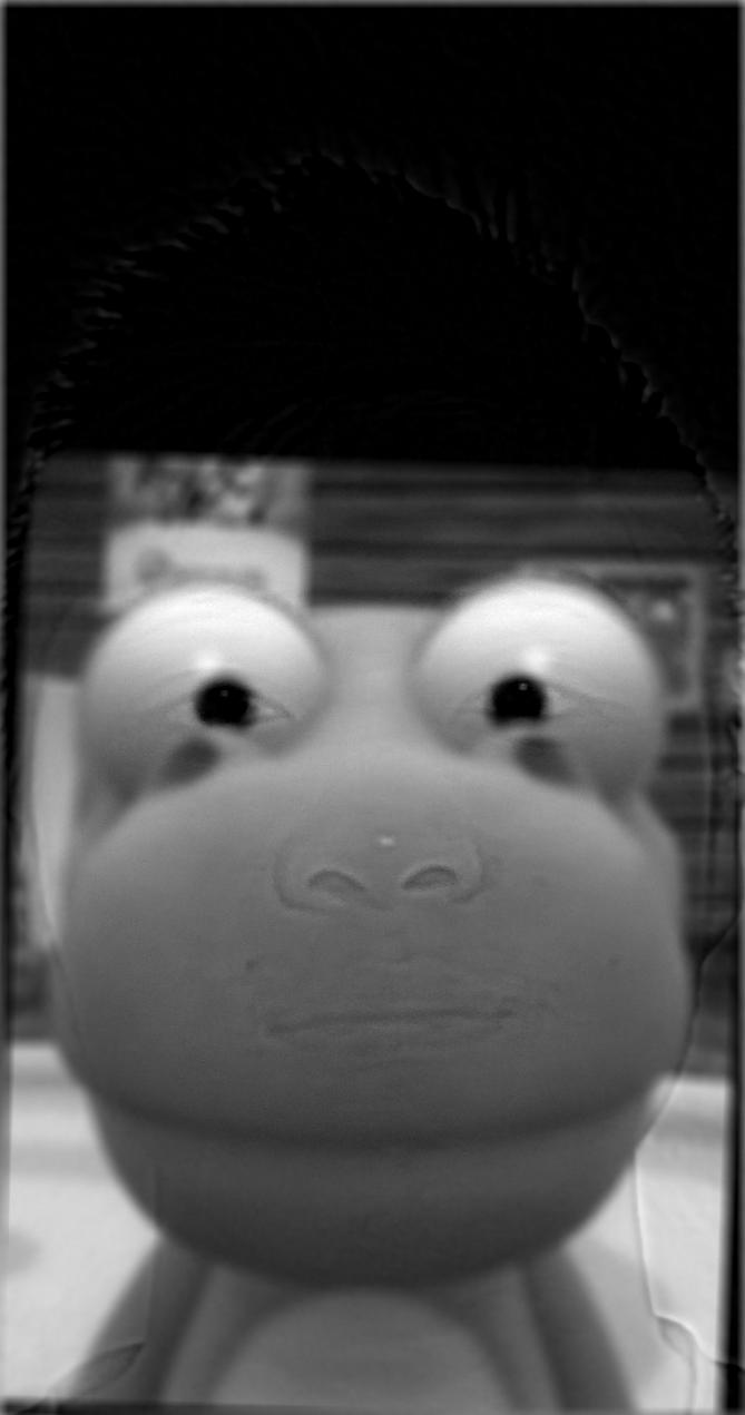
Here is an example of a failed hybridization of my roommate Vincent (taken with permission) and Crong. I believe that this process failed because the image I took of Vincent lacked distinct edges and lines, and thus the high pass filter was unable to pick up on anything distinct to add to the low pass filtered image.

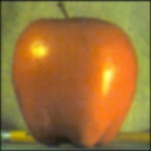
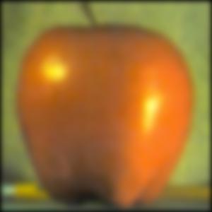
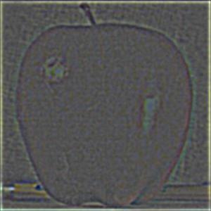
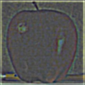
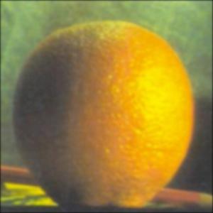
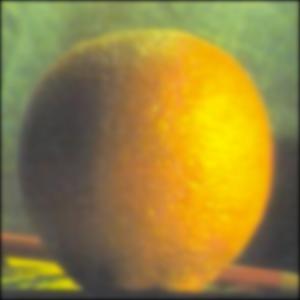
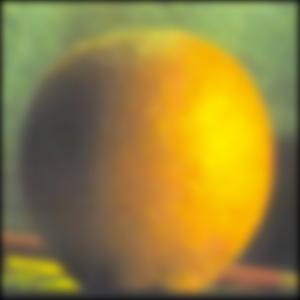
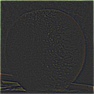
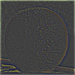
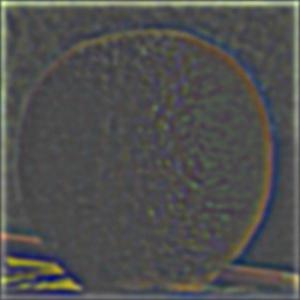
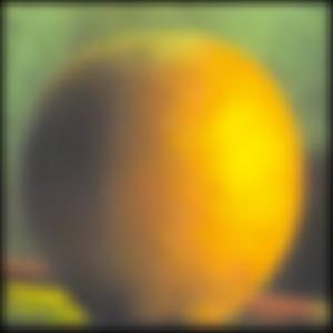
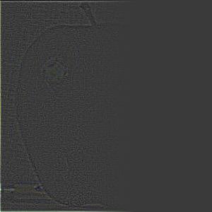
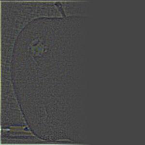
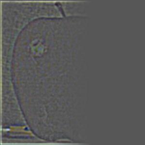
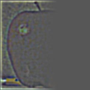
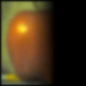
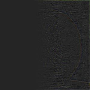
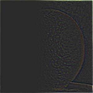
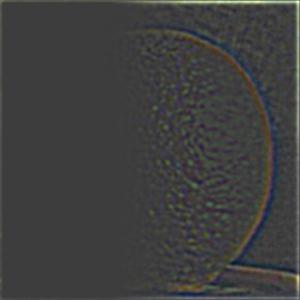
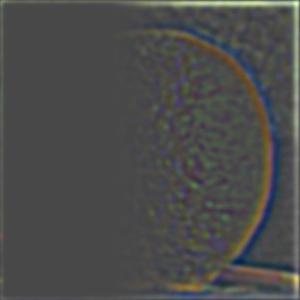
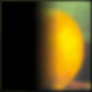
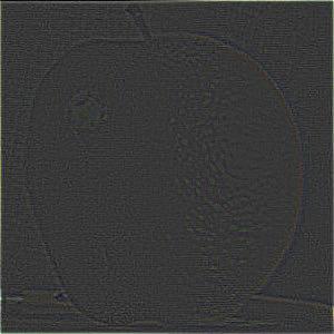
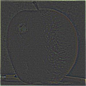
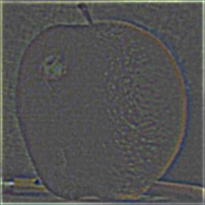
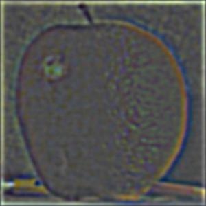
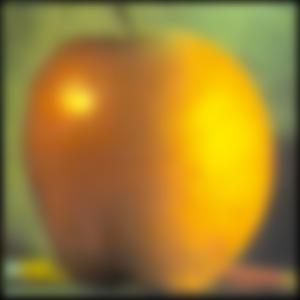
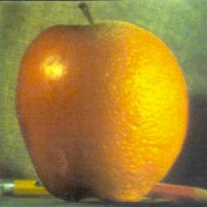
Part 2.3: Gaussian and Laplacian Stacks

In this section, I implemented Gaussian and Laplacian stacks in order to accomodate image blending. As described in the paper, we can combine the Laplacian stack back together into the original image. With this Laplacian stack as well as a Gaussian stack of a mask, we can combine images! Below, I'll show the Gaussian and Laplacian stacks of the Apple first, and then the Orange. I start the first layer using a kernel with ksize=15, and starting sigma=0.5. Then at each successive layer below, I multiply the sigma by 2. I do this for 5 layers.

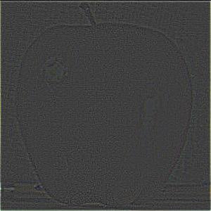
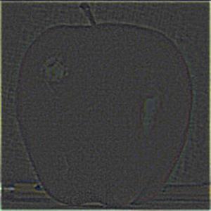
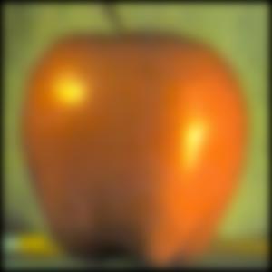
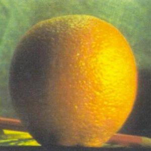
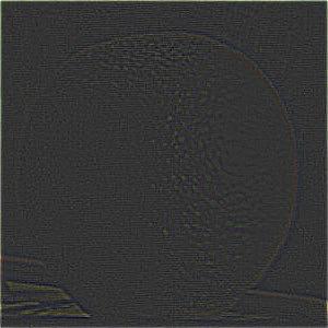
For the next part, I applied the Gaussian and Laplacian stacks to obtain the intermediate components of the Oraple. For reference, these Laplacian stacks are similar to the outcomes in Figure 3.42 on page 167 of the Computer Vision: Algorithms and Applications textbook.

Part 2.4: Multiresolution Blending

Finally I begin to combine images. For creating the Oraple, I created a mask as shown below. I computed Laplacian stacks for the apple and orange each (shown above), as well as the mask's Gaussian stack. For the Gaussian stack for the other image (in this case, the orange), I simply take the corresponding Gaussian in the stack and subtract its values from 1. Below, I show the mask I used, as well as the Oraple result from the process described in project spec. Note that my mask is 0 on one side, 1 on the other side, and then there is a gradient between 0 and 1 from one side to the other.

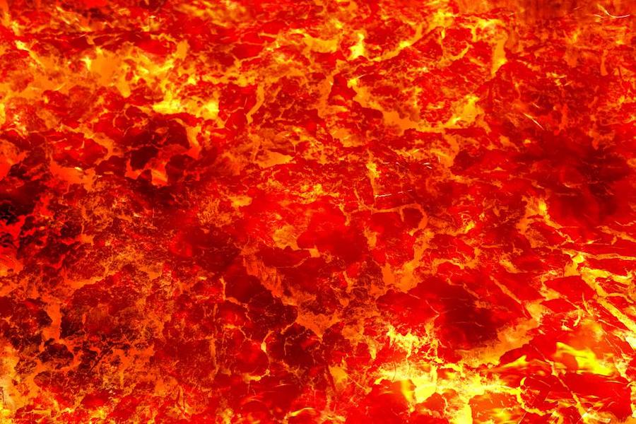
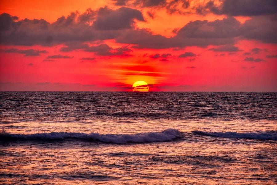
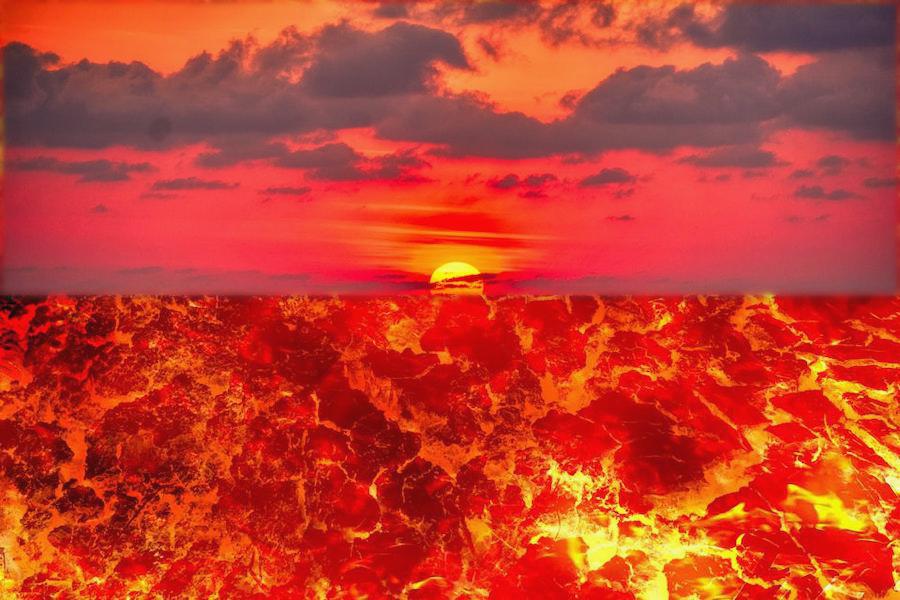
Here's another blending that I attempted. For this one, I'd like to think it looks like the ocean water has been replaced by lava.

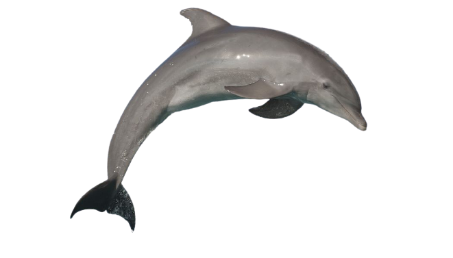
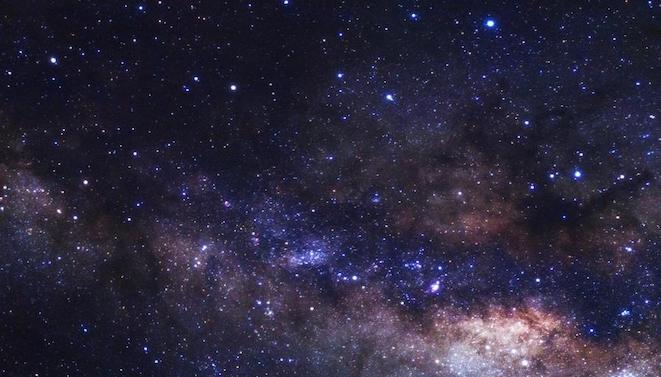
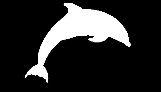
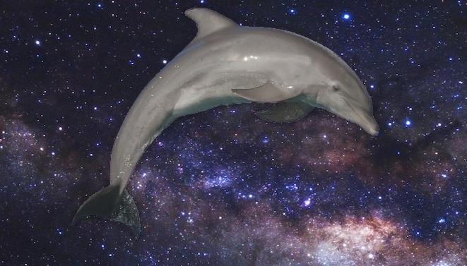
Finally for my last blended image, I put a dolphin into space. Of course, no dolphins harmed in the making of this image.

Reflection

I think this project was really cool, especially in showing how some of the tools in Photoshop work under the hood. I also really enjoyed the hybrid images, with some high and some low filtering that would allow different people to see different things. My roommates really enjoyed my Rock Shrek hybridization.