Fun with Filters and Frequencies

Overview

In this project, I explored several image manipulation methods. First, I implemented edge detection by convoluting images with finite difference operators and Derivative of Gaussian (DoG) filters. Next, I used an unsharp mask filter to sharpen images, and I isolated high and low frequencies in pairs of images to create a hybrid images. Finally, I implemented multiresolution blending with the help of Gaussian and Laplacian stacks.

These exercises showed me that convolutions and Fourier analysis are quite powerful tools for image editing, since human perception is strongly tied to the frequency domain of an image.

Approach

To start off, I wrote some helper functions that would be useful for many parts of the project. One function convolves a kernel over an image to create an identically sized output using a symmetric boundary. It works on grayscale and color images alike. Additonally, I created a function to produce 2D gaussian filters with a σ value always in proportion with the kernel size (such that filter half-width is about 3σ). I used this filter to define blurring and sharpening methods later on. I also added a helper function to remap color intensities to the range [0.0, 1.0].

Part 1.1: Finite Difference Operator

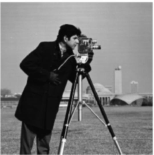
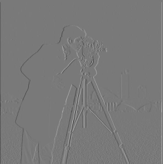
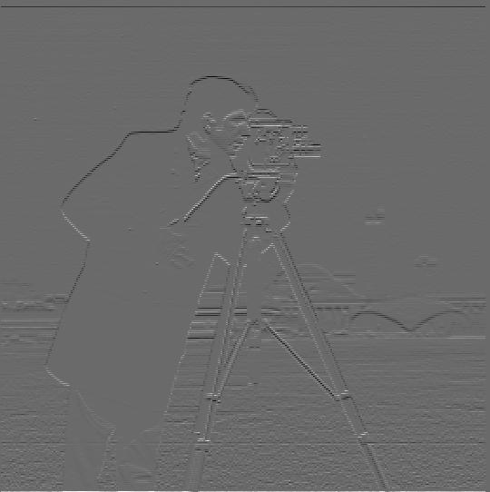
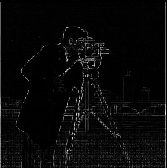
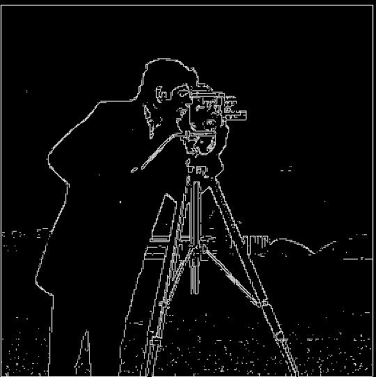
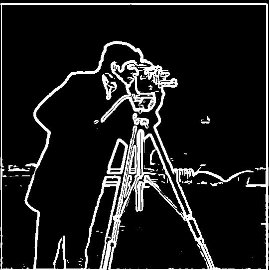
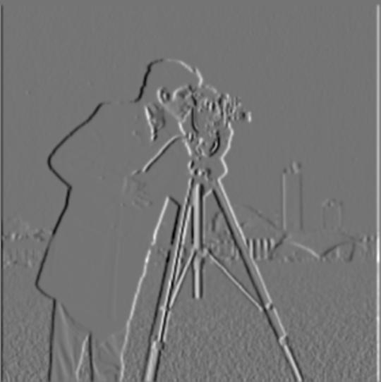
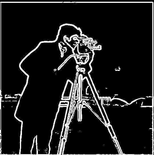
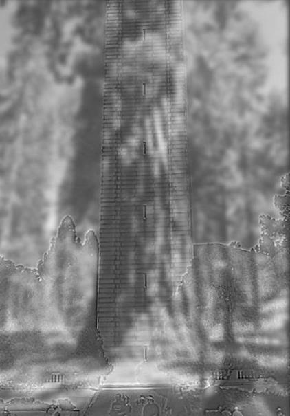
For the first task, I convolved the cameraman image with the Dx and Dy finite difference operators separately to produce partial derivative images, shown in the first row below with colors remaped to center around 0.5 (gray). I then computed gradient magnitude images, one with continuous values and the other binarized for edge detection. This computation involved squaring the partial derivative images element-wise (without remapping) and taking the square root of their sum.

Part 1.2: Derivative of Gaussian (DoG) Filter

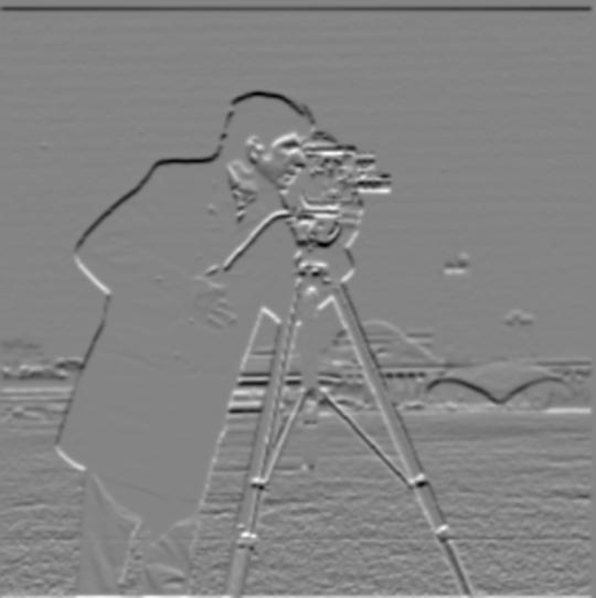
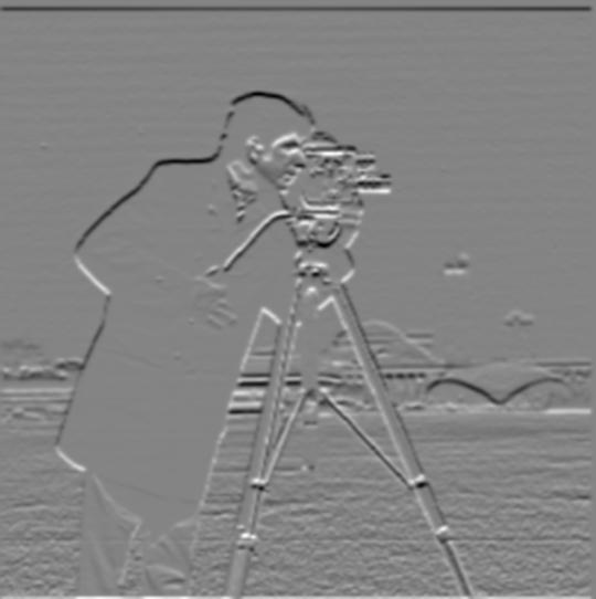
In order to reduce noise in these images, I tried blurring the original image with a gaussian (G), then computing the gradients using the finite difference operators. This process produced the results in the second row below, which were smoother and contained less noise (especially on the grass). The resulting edges outlines are also thicker due to a more gradual change in brightness across the blurred edges. They also appear brighter since I remapped the range of brightnesses to the full range [0.0, 1.0].

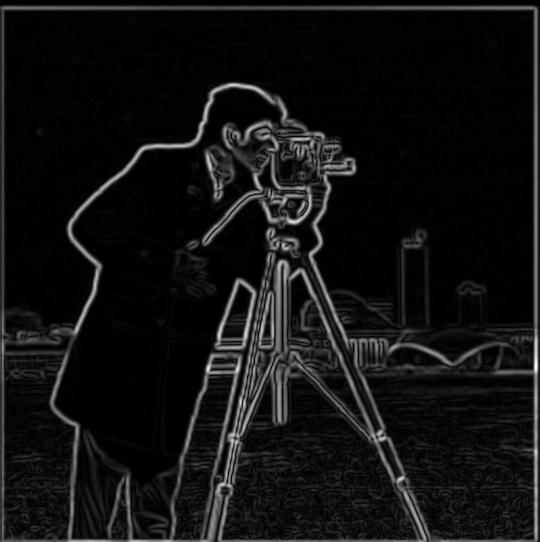
Alternatively, I accomplished very similar results by first convolving Dx and Dy with G to produce DoG filters (shown above). The image could then be convolved with the DoG only once to more efficiently produce nearly identical results, show in the third row below. In all three cases, a binarization threshold of 0.2 was used.

	Dx	Dy	Gradient Magnitude	Gradient Binarized
Original (1.1)
Pre-Blurred (1.2)
DoG Filter (1.2)

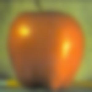
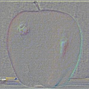
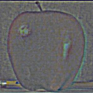
Part 2.1: Image "Sharpening"

For this part, I created an unsharp mask filter. The parameter α was used to control the amount of "sharpness" added. The gaussian was scaled -α, while the impulse kernel was scaled by (1 + α). These two scaled kernels were then added together and convolved with the image once to produce the sharpened version. Some clipping was necessary to constrain the brightness values of all pixels to the range [0.0, 1.0].

α = 0.0 (original image)	α = 1.0	α = 2.0	α = 5.0

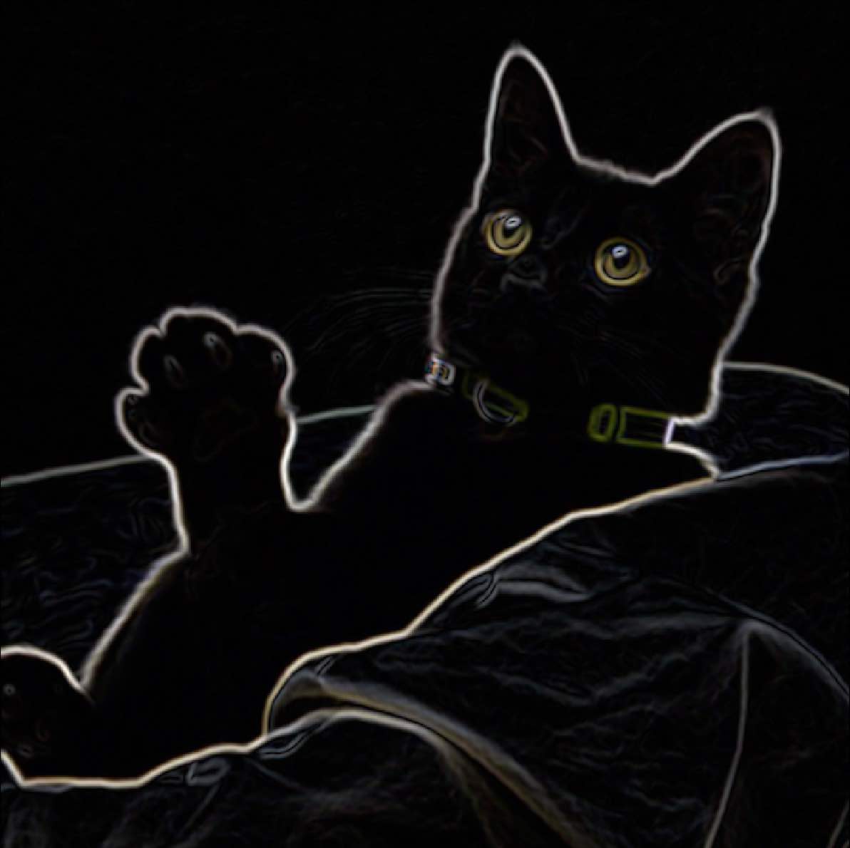
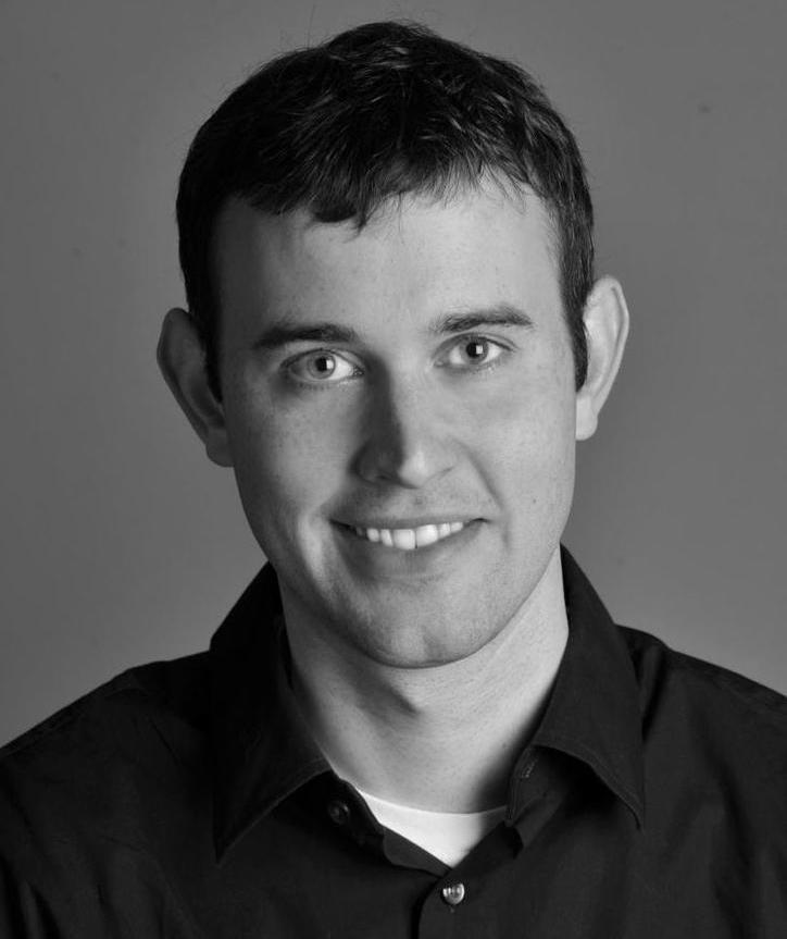
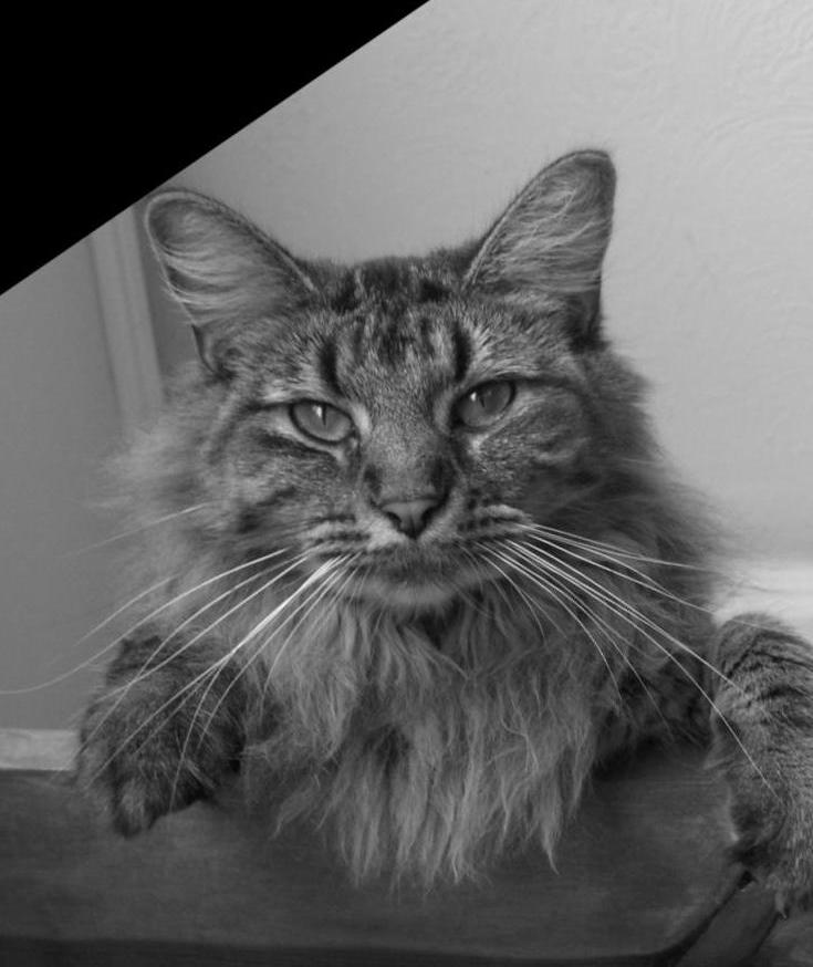
For the image below, I tested what would happen if I blurred the original image and attempted to restore sharpness via the unsharp mask. With an α value of 10.0, the major edges (cat outline, large patterns on bed) regained much of the sharp definition they had lost due to blurring. However, the fine details of the cat's fur weren't faithfully reconstructed, especially on the face. The unsharp mask filter cannot effectively restore the highest frequencies lost due to blurring, it only emphasize the high frequencies that remaining intact.

α = 10.0 (closest match to original)	α = 0.0 (original image)	α = 0.0 (blurred image, 10x10 gaussian)
α = 1.0	α = 2.0	α = 5.0

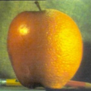
Part 2.2: Hybrid Images

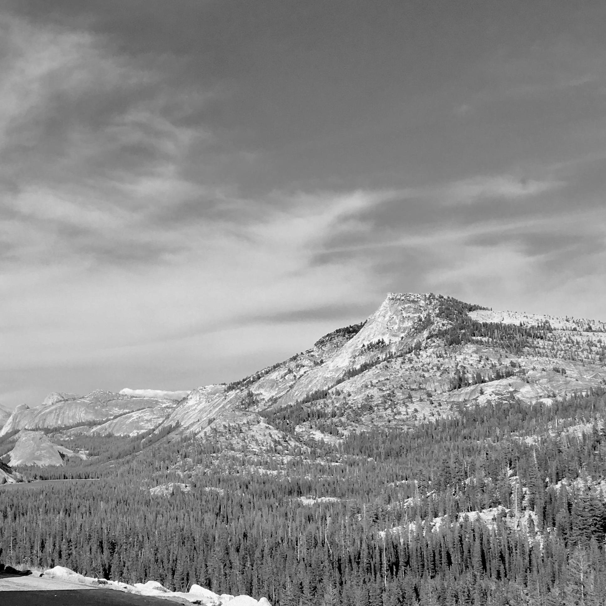
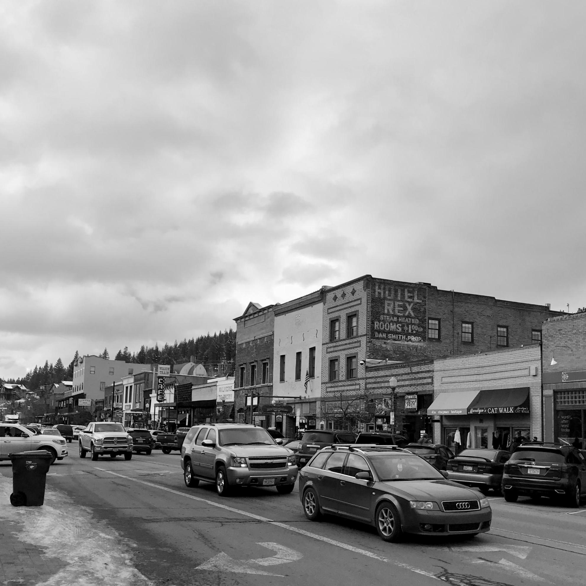
A hybrid image is a the combination of two filtered images, one showing only the low spacial frequencies (gradual changes in brightness), the other showing high frequencies (edges and smaller details). I chose the pair of images so that the large-scale composition of objects were similar.

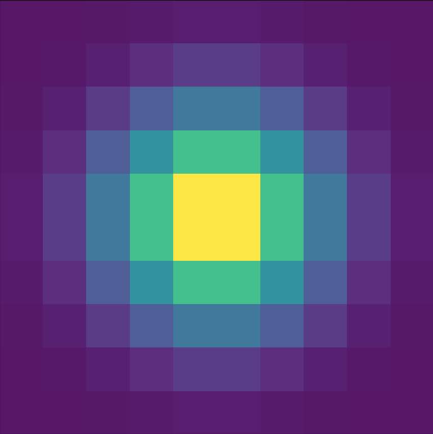
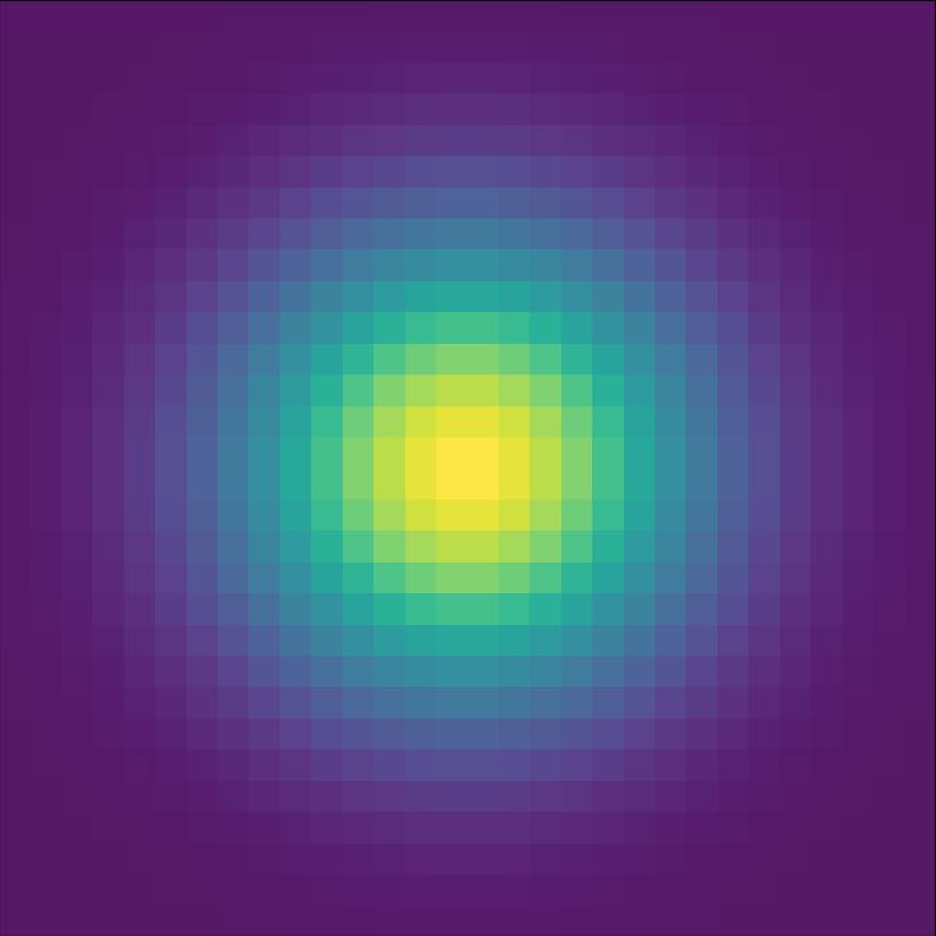
For my lowpass filter, I used a standard 2D Gaussian. For the highpass, I used a unit impulse filter minus a Gaussian. The cutoff frequencies of each filter varied depending on the pair of chosen images

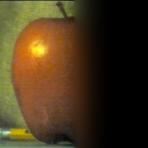
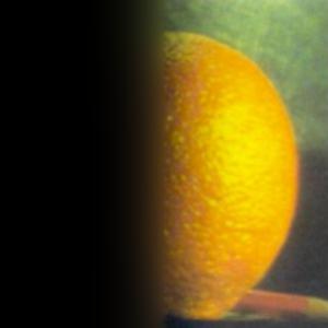
Low frequency source	Lowpass	High frequency source	Highpass

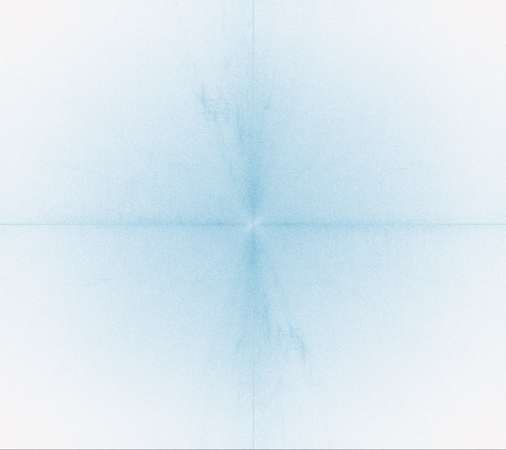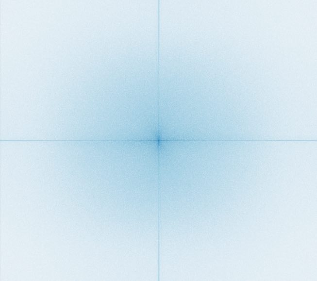
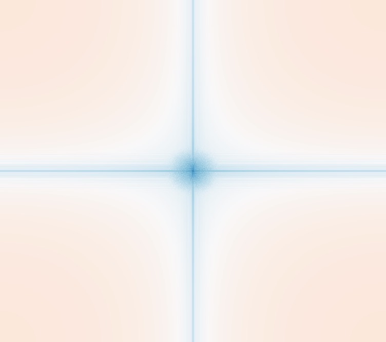
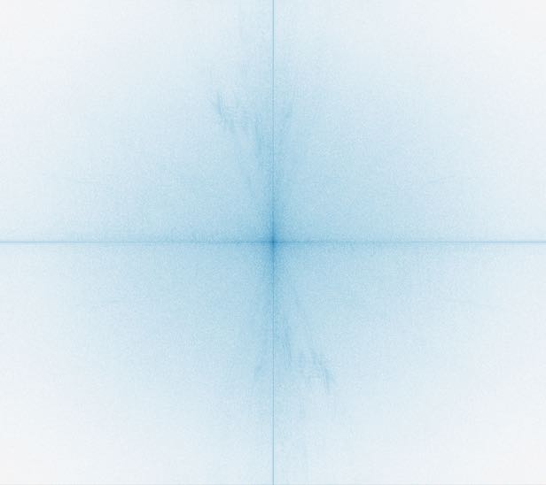
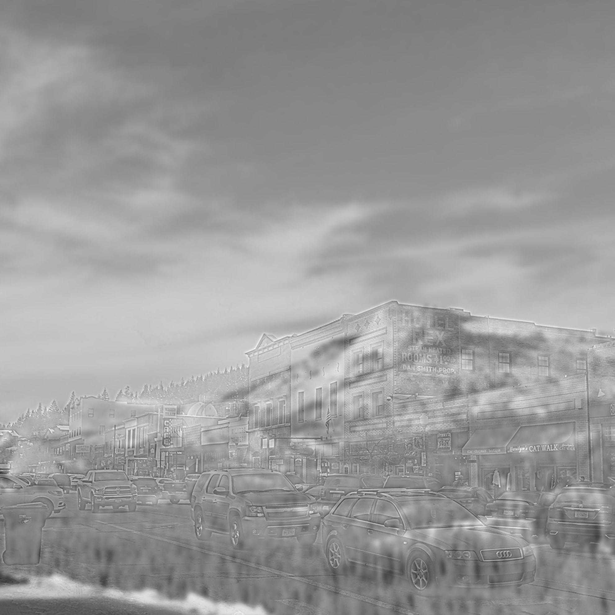
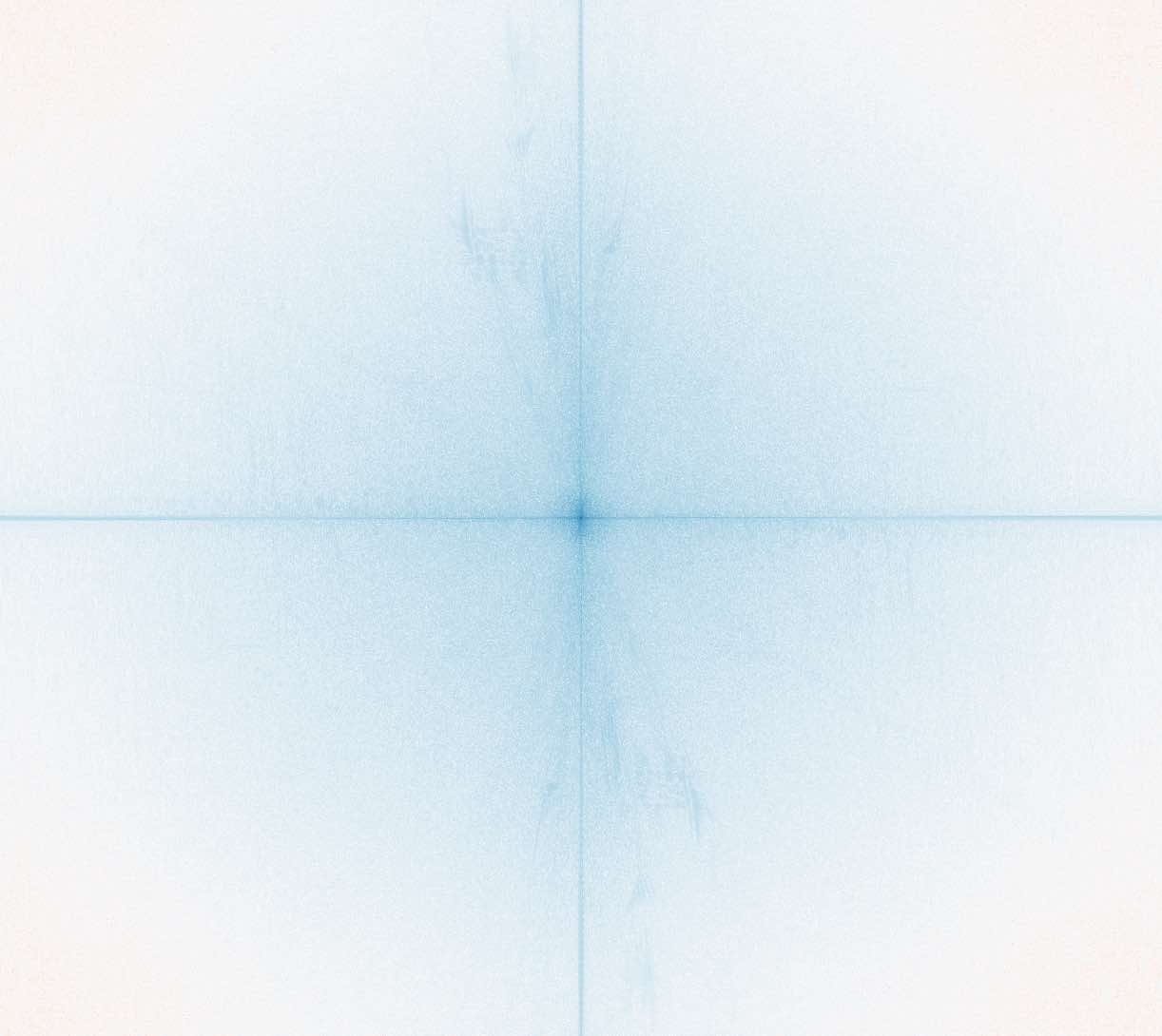
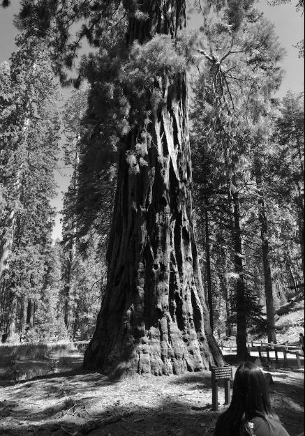
Above, I've shown the fourier transforms of the images I chose for one of the hybrid images, in their original and filtered forms. Darker blues refer to a greater presence of that frequency, with low frequencies near the center. As you can see, the lowpass (blur) filter on the Yosemite image removed much of the higher frequencies, but left intact the low frequencies near the origin of the frequency space image. On the other hand, the highpass filter on the image of downtown Truckee, CA reduced only the low frequencies close to the center of the frequency space image. The resulting hybrid image, shown below with its Fourier transform, is the element-wise average of the two filtered images.

Hybrid image	Fourier transform

Additional hybrid image results are shown below, along with their two source images.

Low frequency source	High frequency source	Hybrid image

Part 2.3: Gaussian and Laplacian Stacks

In order to implement multi-resolution blending, I first needed to create Gaussian and Laplacian stacks of my images. A Gaussian stack is simply a sequence of successively more blurry images, but all images have the same dimensions. I created this stack recursively, blurring the image with a lowpass (Gaussian) filter that doubled in size at each level of the stack (stopping once the filter height surpasses the image height). The farther down the stack, the lower the maximum frequency of the image.

Gaussian Stack of Apple

The Laplacian stack was computed as the difference of successive Gaussian stack images, resulting in a series of images representing a band of frequencies. The last image in the Laplacian stack is simply the lowest frequency Gaussian stack image, so that adding all images in the Laplacian stack will reconstruct the original image.

Laplacian Stack of Apple

Szelski Figure 3.42 (Laplacian Blending)

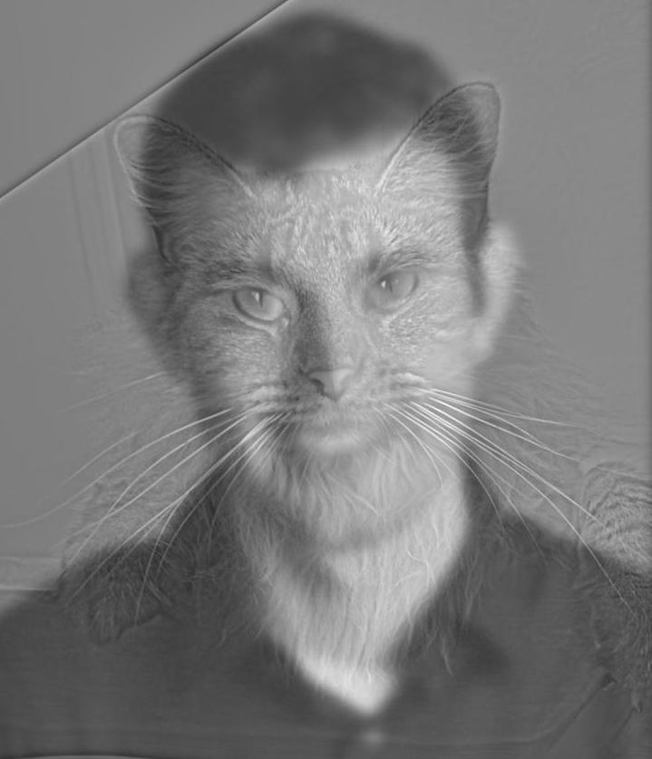
Part 2.4: Multiresolution Blending

The first step in multiresolution blending is to create Laplacian stacks for the two images, as well as a Gaussian stack for the mask itself. The mask controls which of the two images is visible at each pixel on the blended image, with a smooth transition between the two. The lower in the stack, the more gradual the transition from white to black, corresponding to a smoother blend.

Gaussian Stack of Vertical Seam Masks

For each level in the Laplacian image stacks, the corresponding left-side mask is multiplied element-wise with the left-side image, corresponding right-side mask is multiplied element-wise with the right-side image, and the two sides are added together to get a blended Laplacian stack. Finally, all levels of this stack are added back together to get the final blended image!

Gecat Laplacian Blending

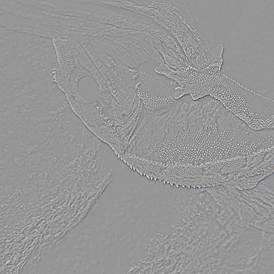
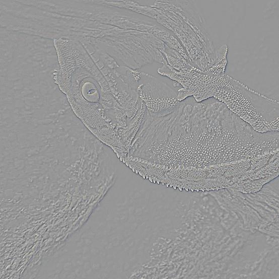
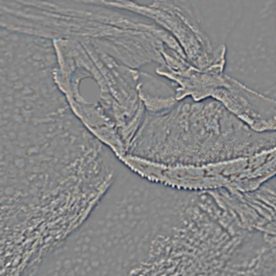
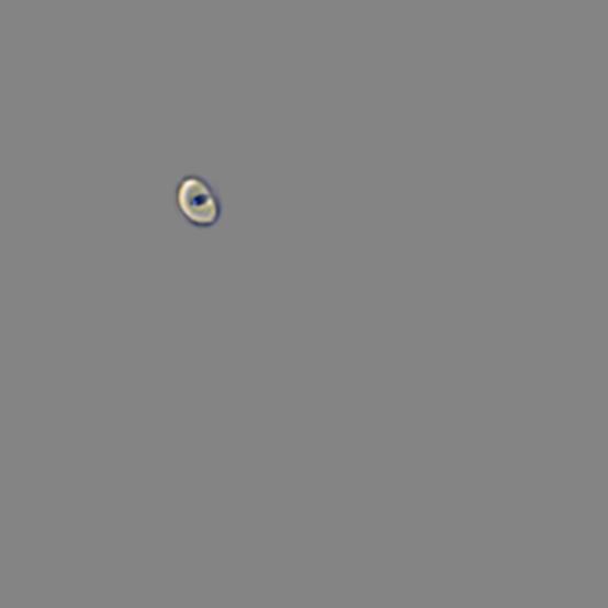
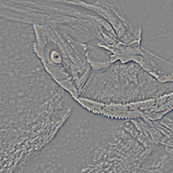
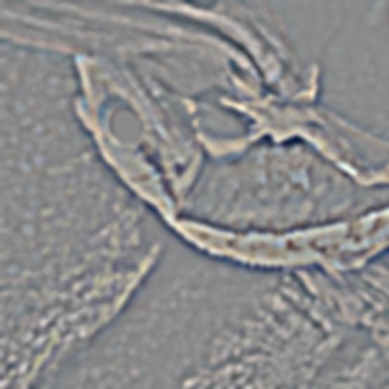
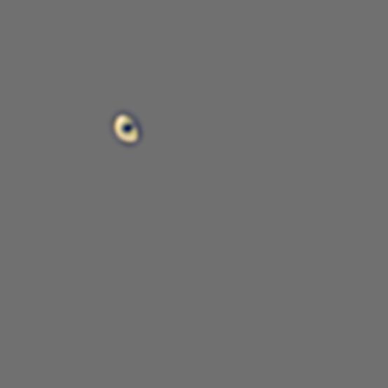
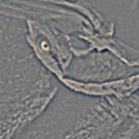
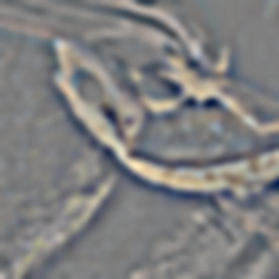
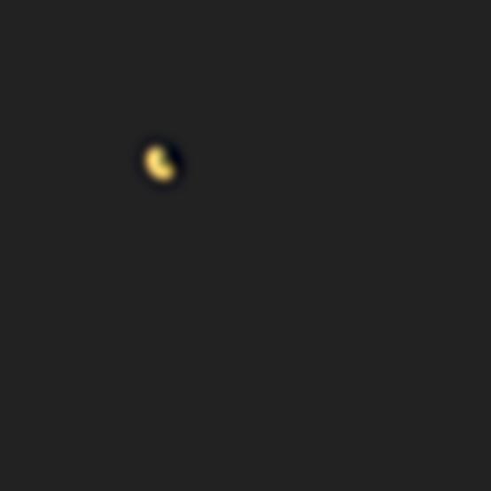
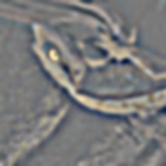
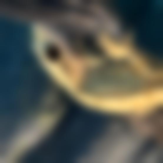
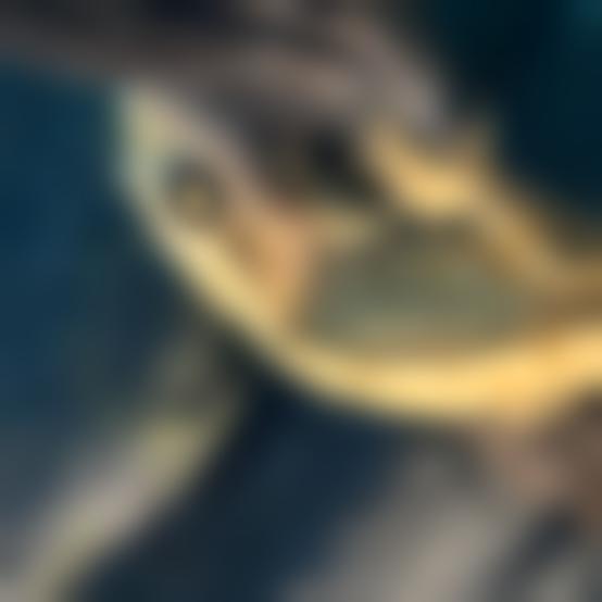
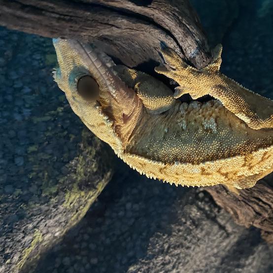
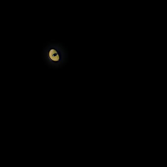
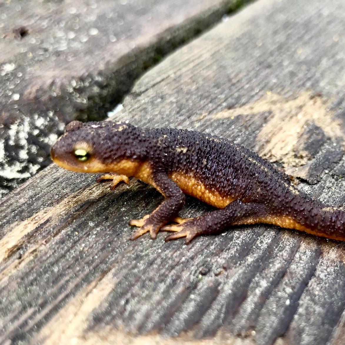
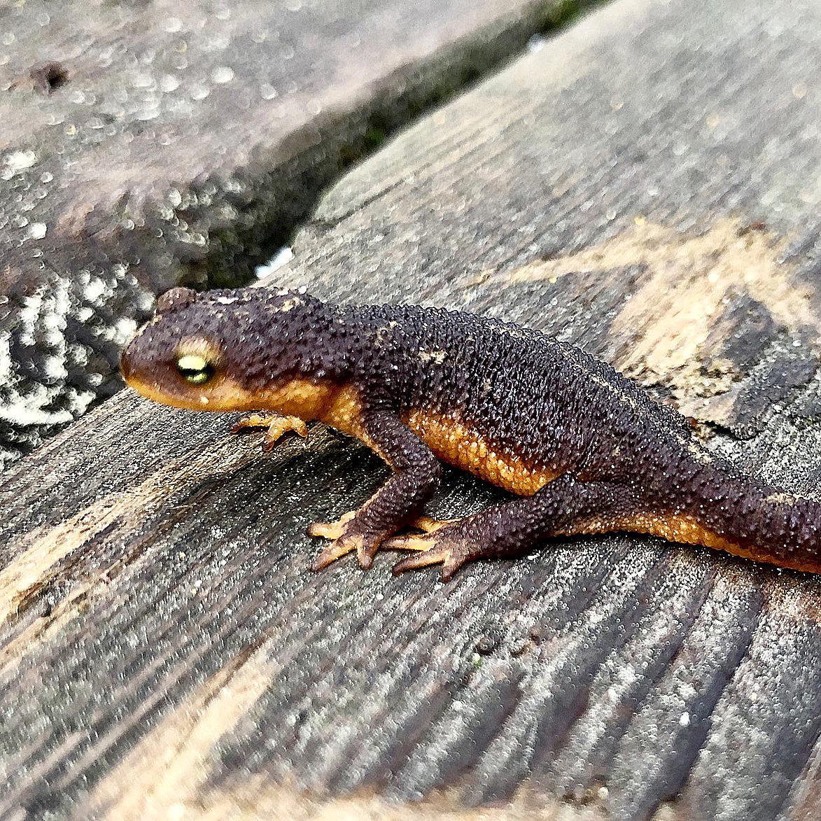
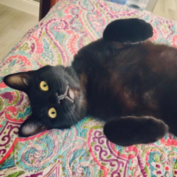
In the example above, I placed the eye of my cat, Ollie, onto the face of my gecko, Nugget. I've shown the blended result for each resolution layer, as well as the final result.

Apocalypse Day Laplacian Blending

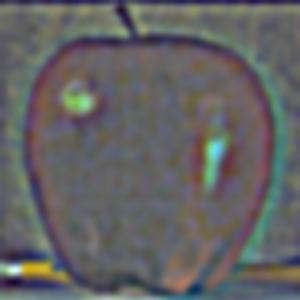
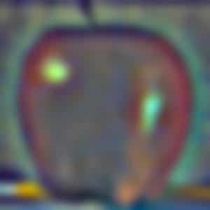
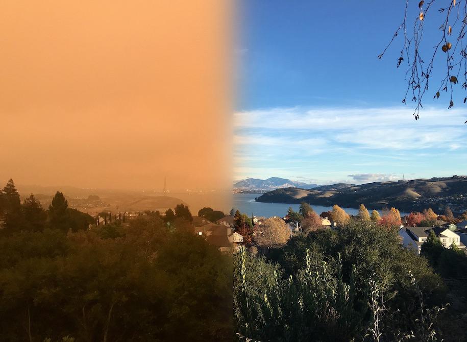
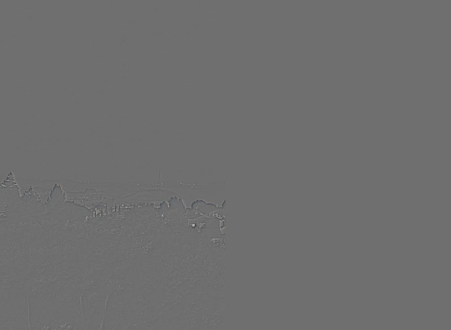
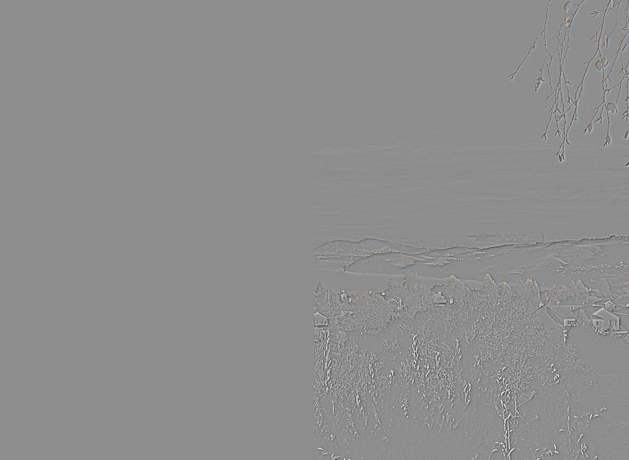
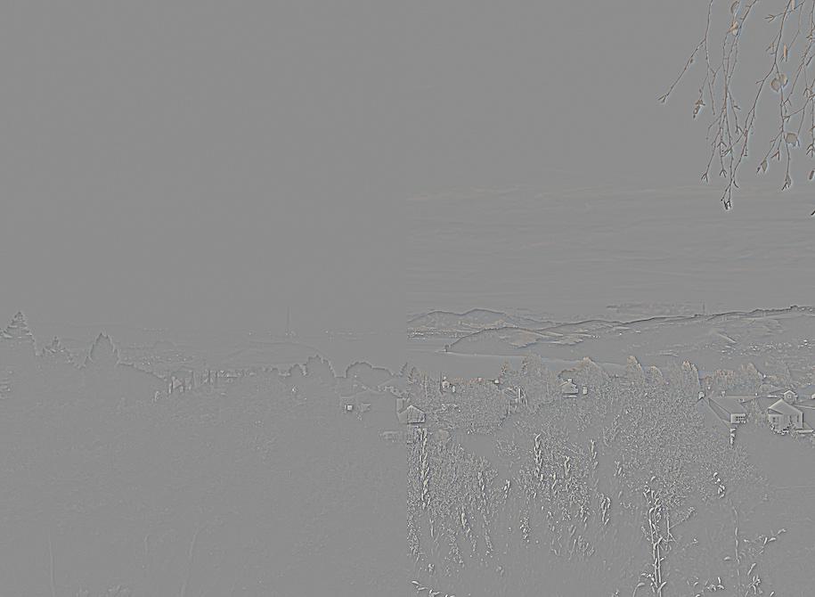
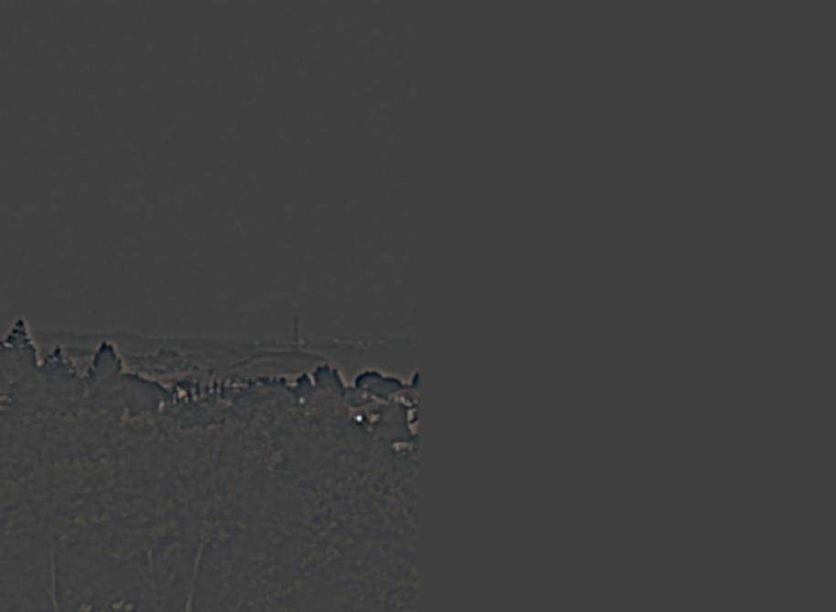
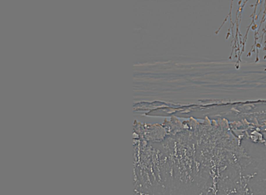
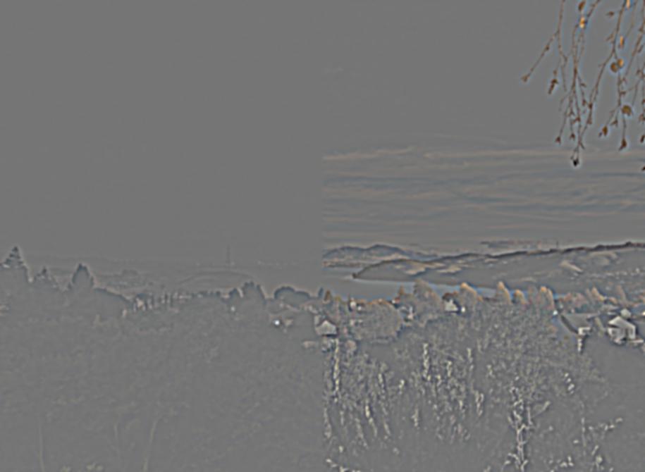
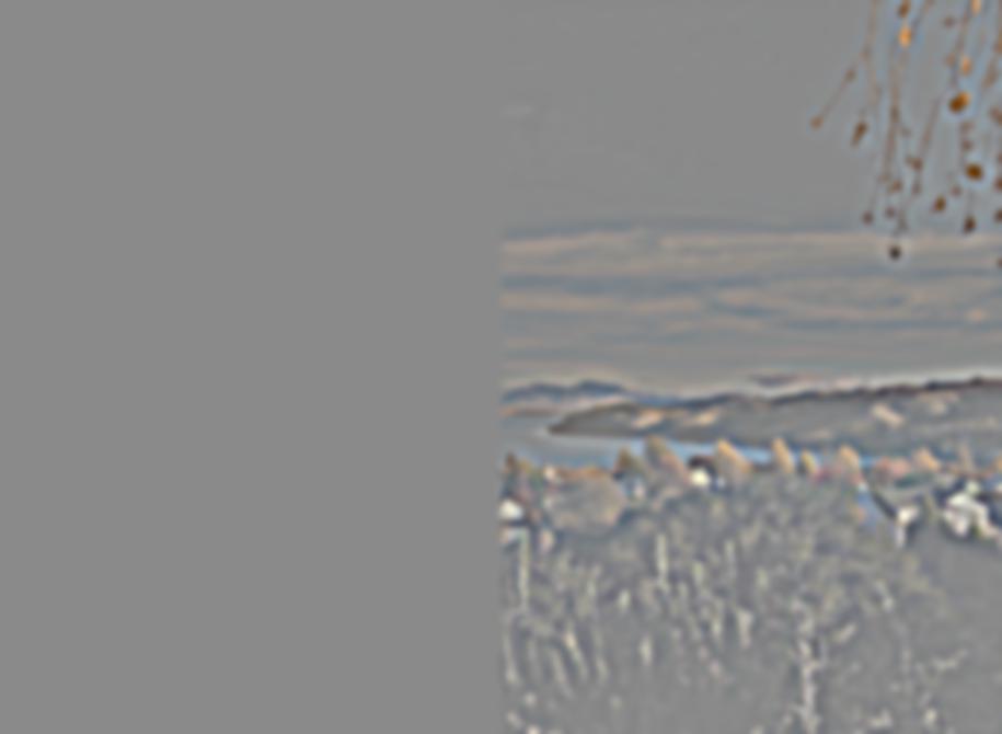
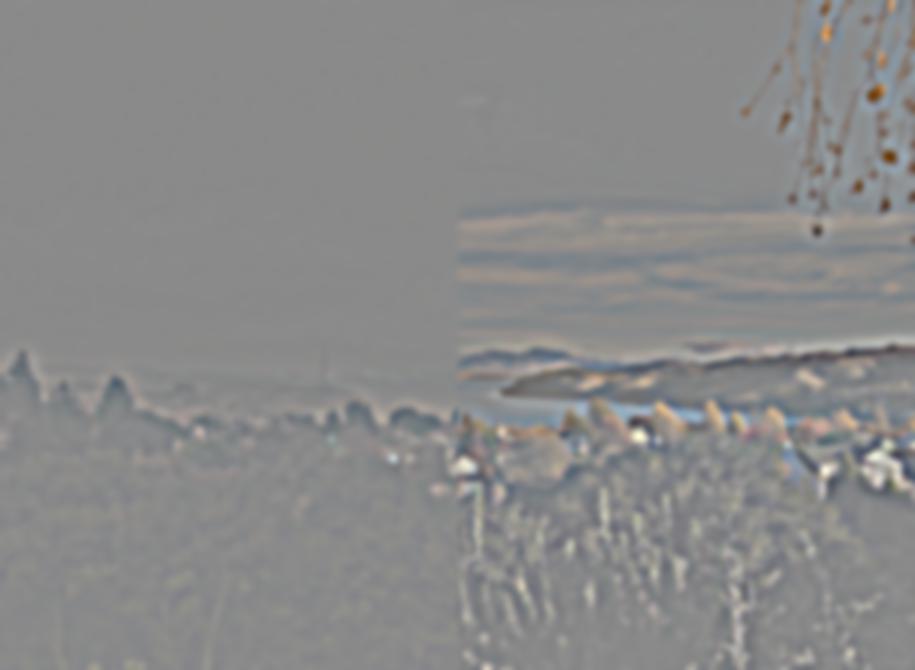
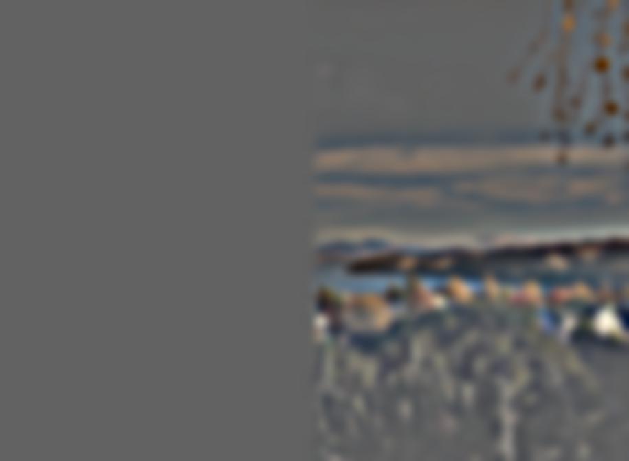
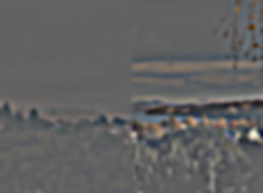
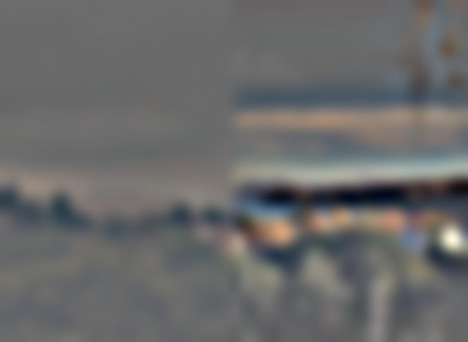
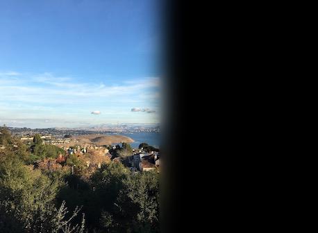
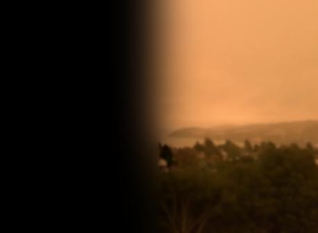
For my last example, I blended an image of the view from my parent's back patio on a nice day with that same view on 9/9/20 (that time the sky was dark and orange the entire day, which also happened to be my 20st birthday!). I wasn't completely happy with this result, because the method of blurring made the high frequencies of the plants of the right side abruptly end when they reached the left side, which feels a bit jarring in this context.

Overall, I learned that filters and spacial frequency analysis are extremely useful for image manipulation. I was surprised by the strong ties between human visual perception and the frequency domain of an image.