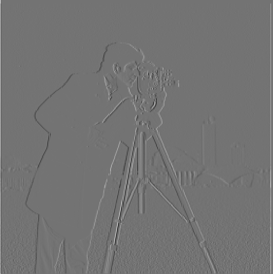
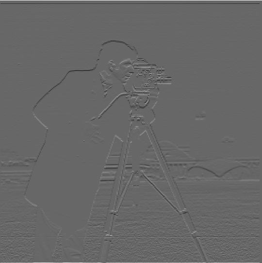
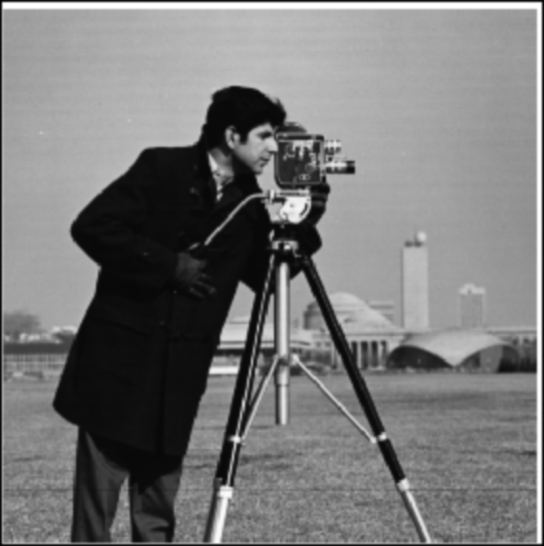
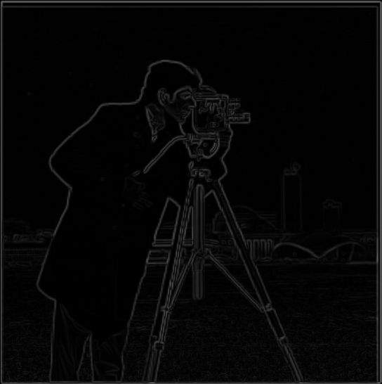
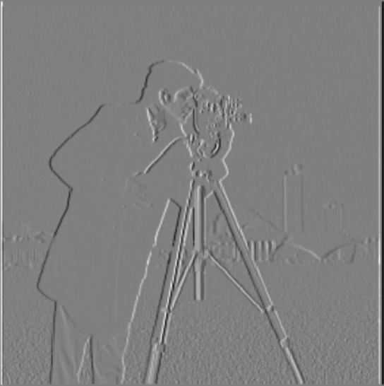
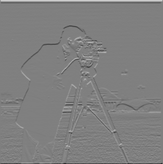
First, I convolved the image with D_x and D_y to produce the partial derivatives. w.r.t. x and y
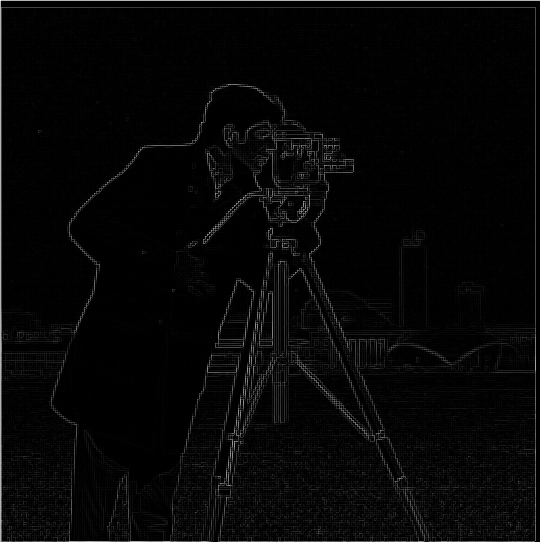
Then, I squared each partial, summed, and took the square root to get the gradient magnitude, as described in lecture.
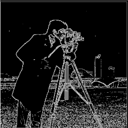
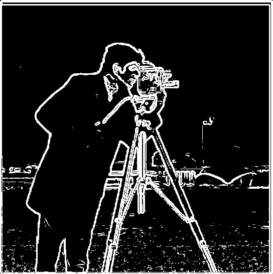
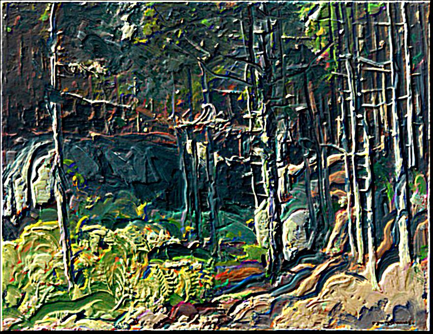
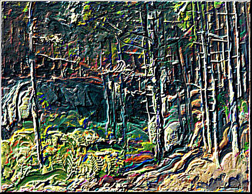
Then I binarized the gradient magnitude to try and show the edges more clearly, with less noise.
I convolved the image with a 2D gaussian kernel to blur the image:
For this blurred image, I computed dx, dy, gradient magnitude, and binarized gradient magnitude as before:


What differences do you notice?
I notice that for the binarized edges on the blurred image, the lines are a lot smoother, there are less artefacts. For instance the background is pretty much all black, previously it had white specks.
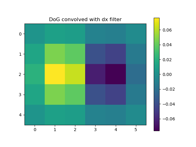
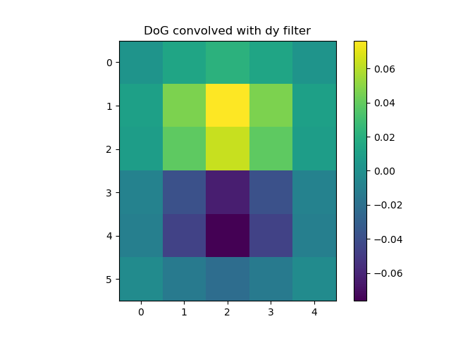
Then I convolved the Gaussian filter with d_x and d_y to get a single filter to apply to the original image, to see if we can get same results with one convolution only.
They look the same as the results above for dx and dy.
Here are filters that I obtained from convolving the gaussian with d_x and d_y
From lecture, we know that you can compute the sharpened image by subtracting the
blurred image from the original image to get high frequencies, and add this
to the original image.
We can combine this into a single convolution by computing the filter:
(1 + alpha) * e - alpha * g
where:
e is unit impulse (identity)
g is the gaussian
and "*" represents the convolution operation
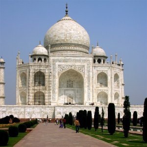
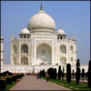
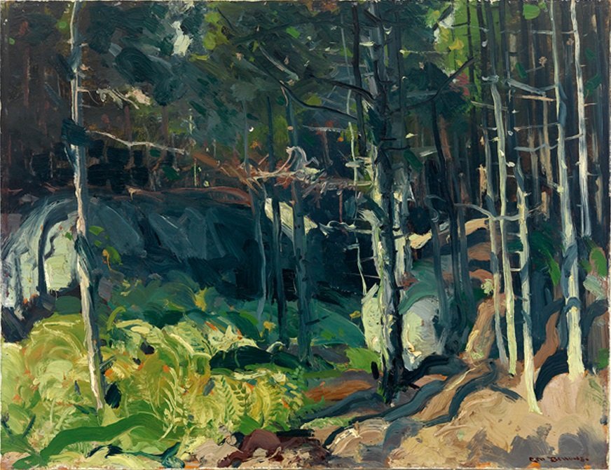
To evaluate this filter, we pick a sharp image, blur it, try to sharpen again. I tried sharpening with a range of different alpha values.
original
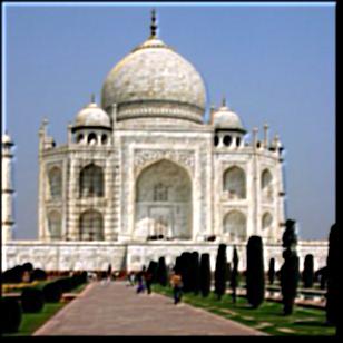
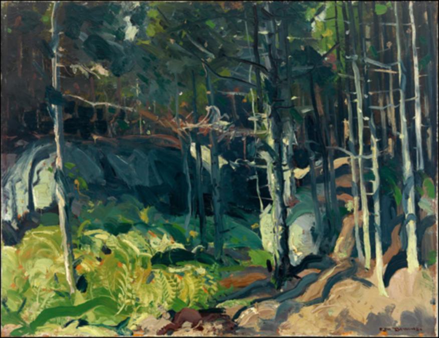
blurred
alpha=1
alpha=5
alpha=10
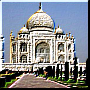
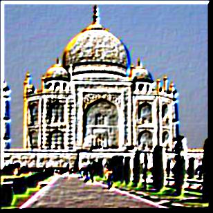
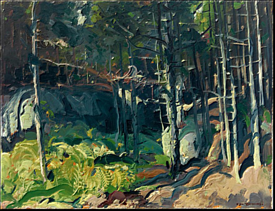
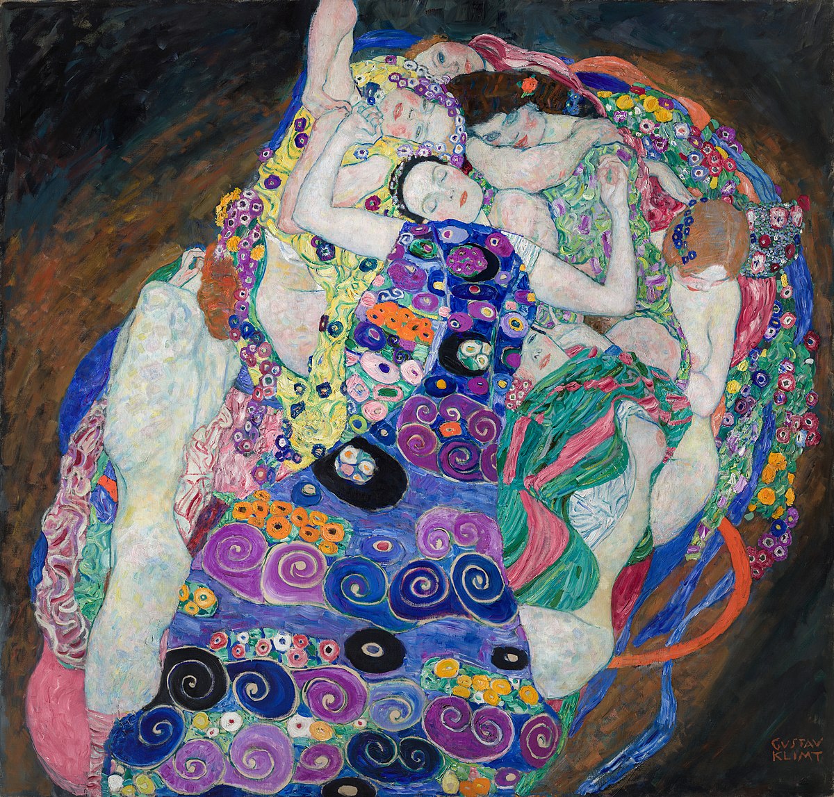

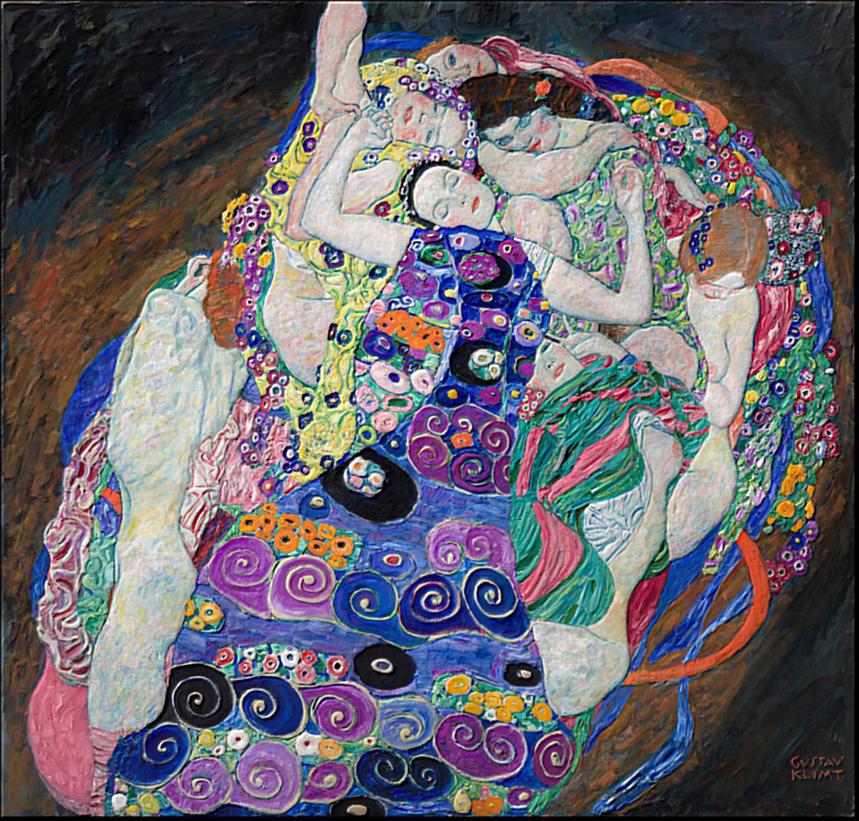
My observation: using this sharpening mask does not seem to be able to recover very small / fine-grained details of the origianl image, it is more like it increases the contrast of the major lines / details - as you increase the alpha, the effect gets stronger and the images appear to be almost "solarized".
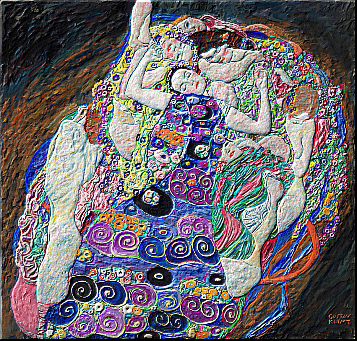
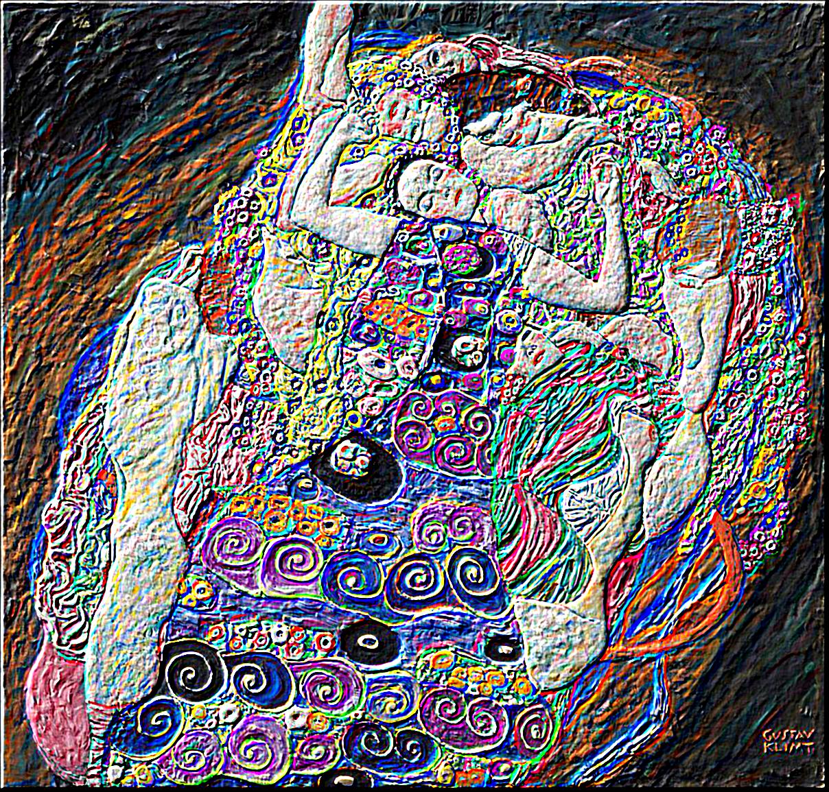
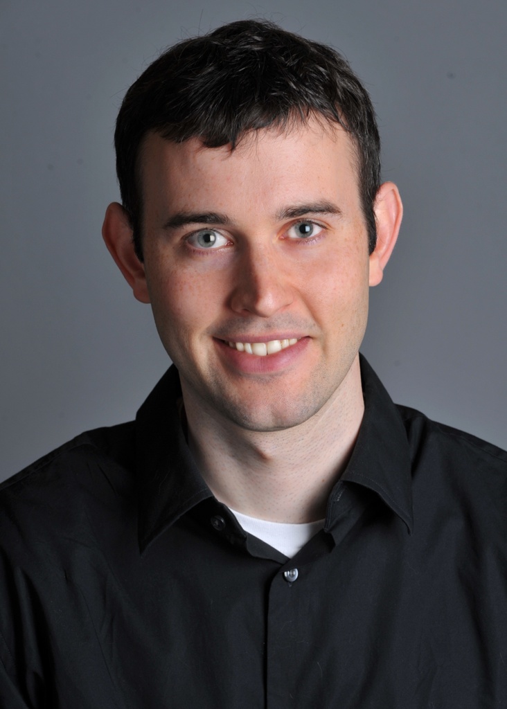
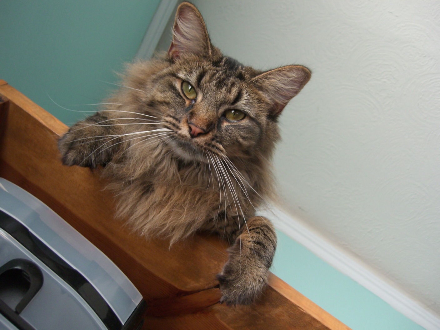
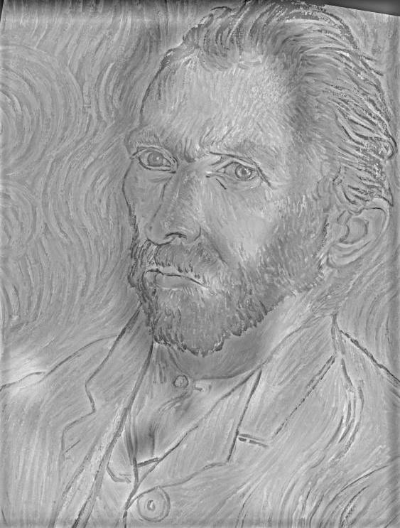
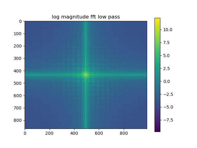
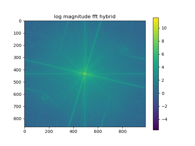
To create hybrid images that look different at different viewing distances, we take two images, "low pass" one of them with a gaussian, and "high pass" the other by subtracting the gaussian filtered image from the original. Then I averaged these two filtered images to create the hybrid.
First, hybrids in grayscale:
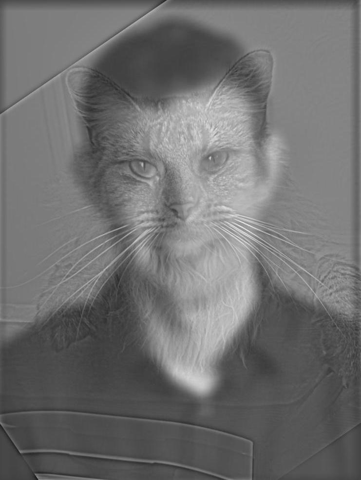
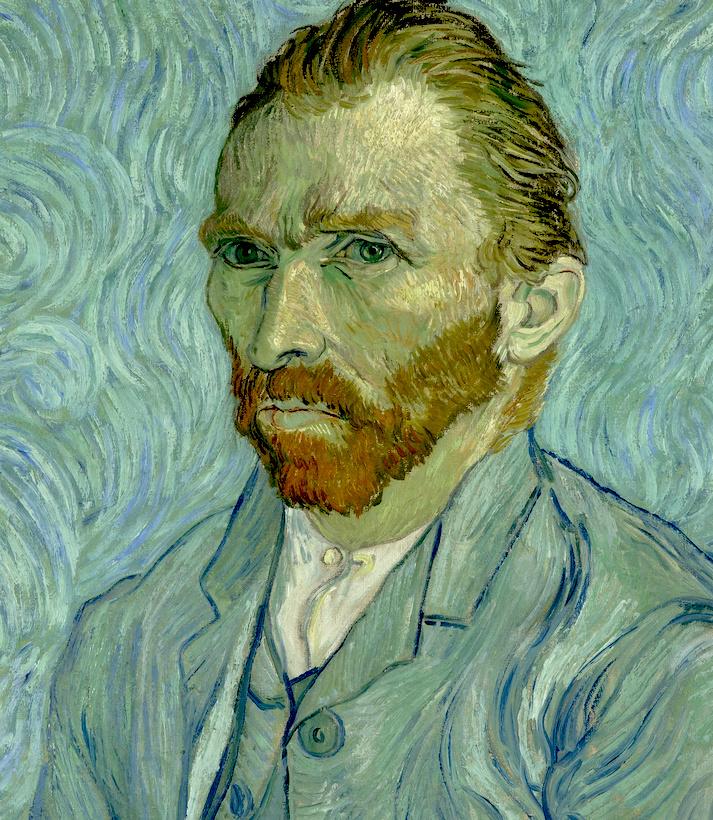
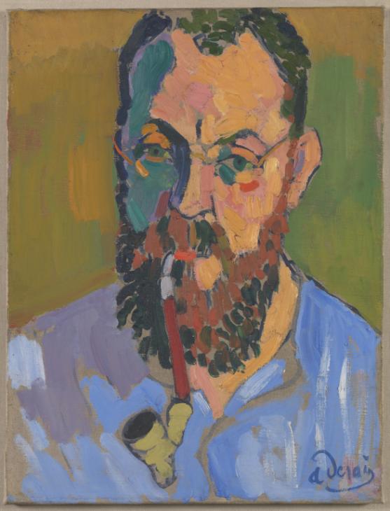
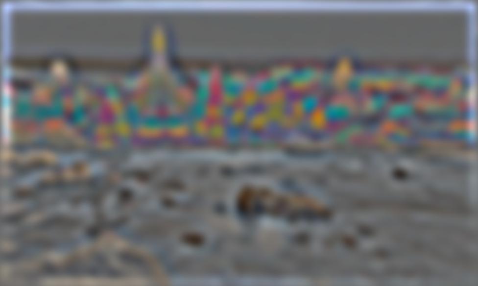
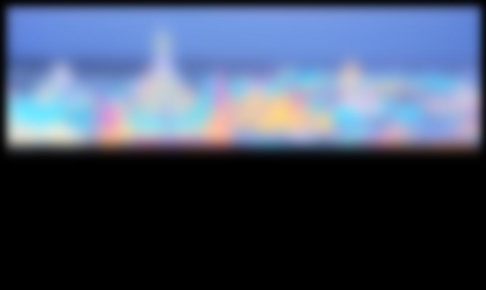
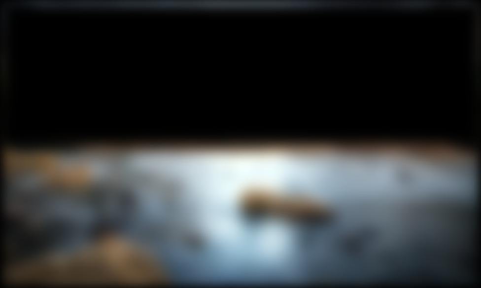
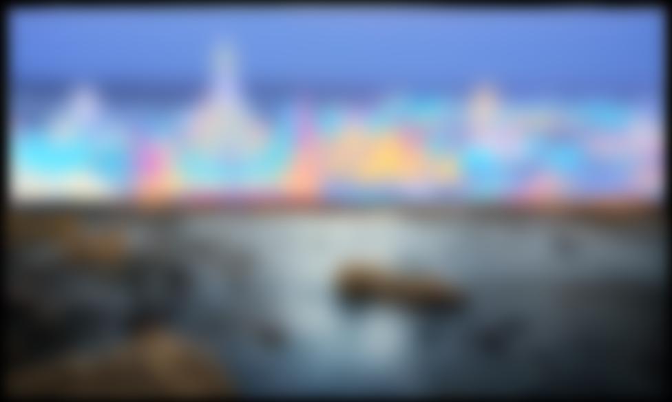
Now for the bells and whistles, hybrid in color:
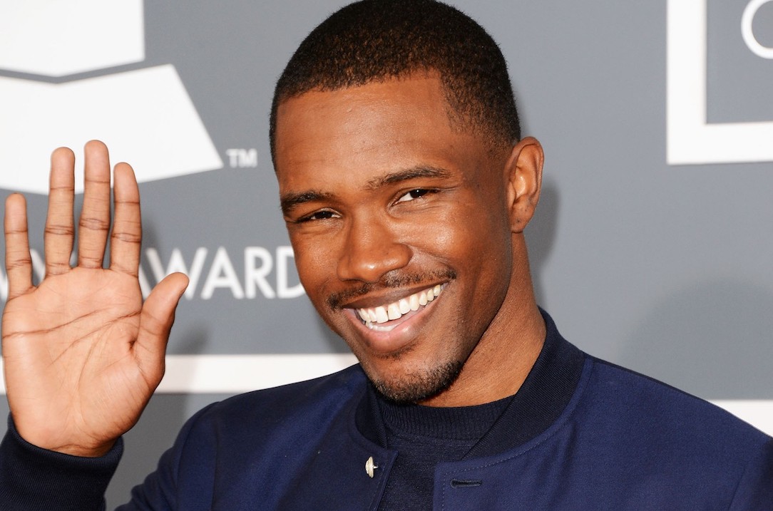
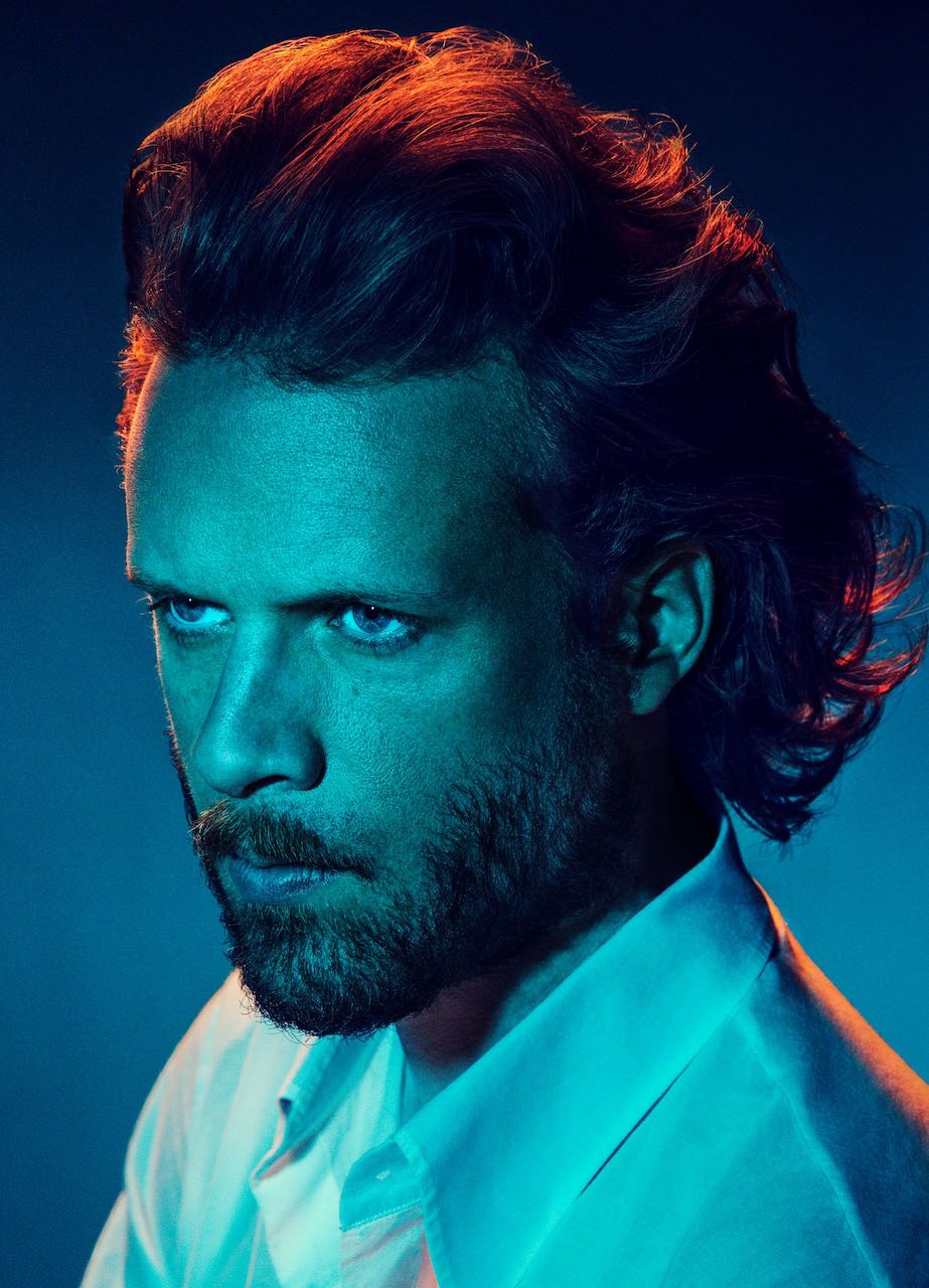
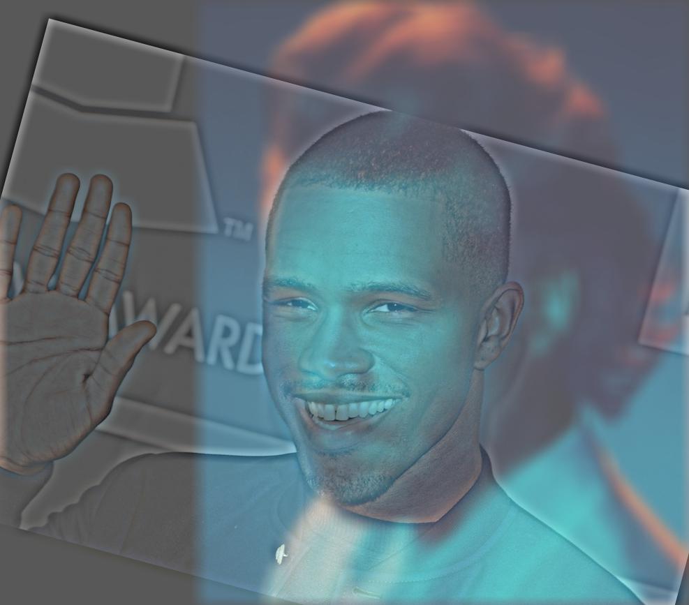
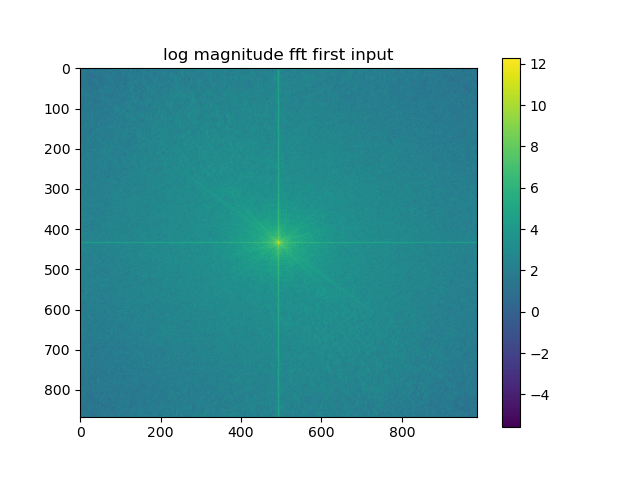
I liked the father john ocean hybrid the best, so I displayed the analysis with fourier transforms for this result:

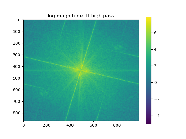
Overall, I noticed that for the effect to show up well, the objects had to have similar structures and shapes. Because I used either portraits or faces this also made the images easier to align. I did think the color on the high pass image got washed out a lot as well, for instance you can only see faint colors around Frank's ear as the FJM image is way more vibrant.
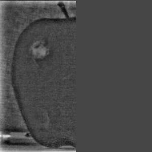
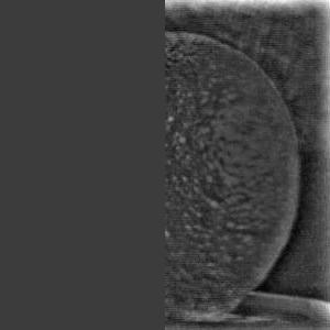
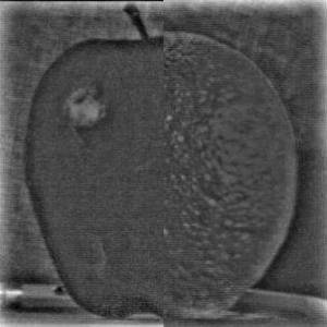
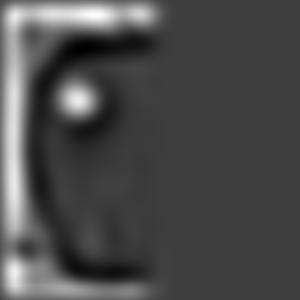
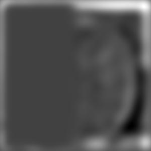
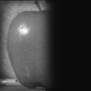
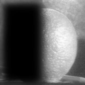
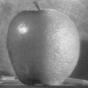
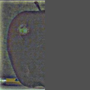
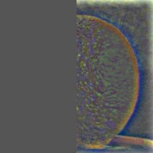
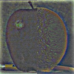
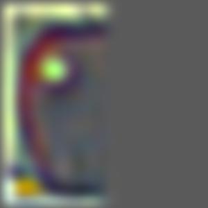
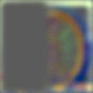
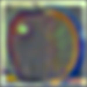
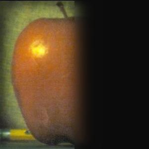
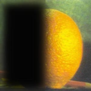
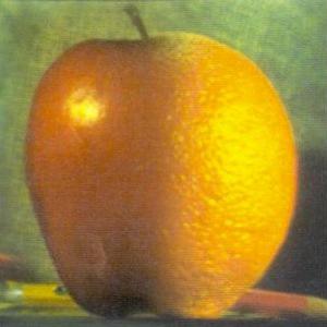
I implemented Gaussian and Laplacian stacks for the orange and apple and blended
together using a vertical seam. The gaussian stack is
the same Gaussian filter (kernel size = (30, 30), sigma=10) successively to
the original image. The laplacian is constructed from the difference of
the i and i+1th image in gaussian stack. Last level of laplacian is last
level of gaussian so we can reconstruct original images by summing Laplacians.
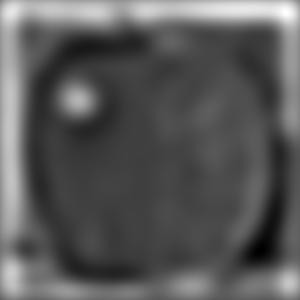
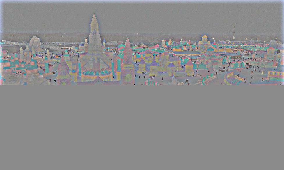
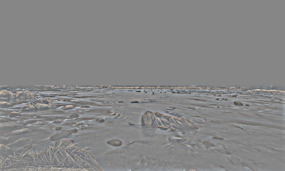
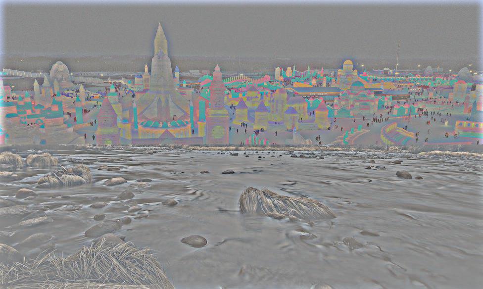
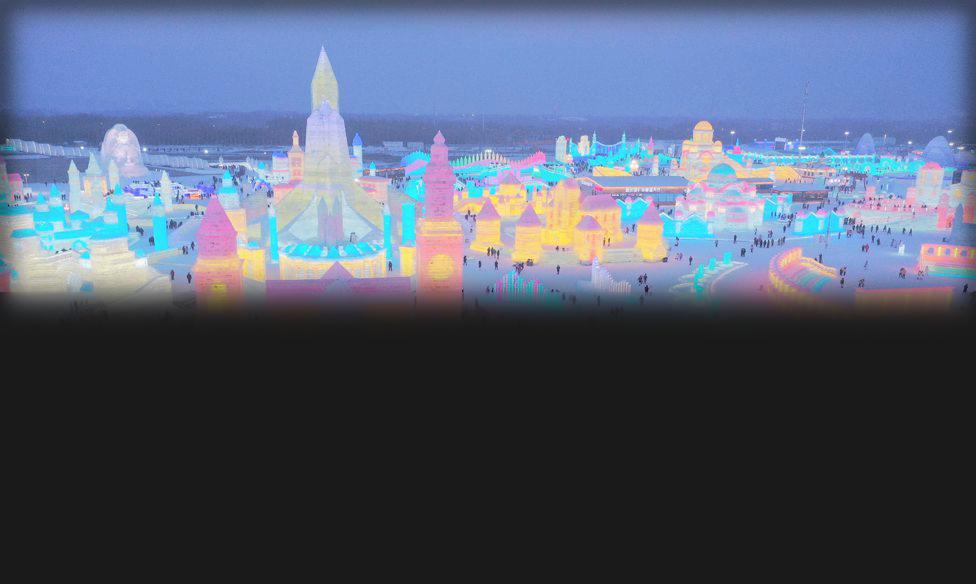
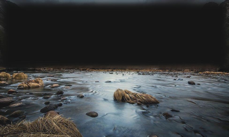
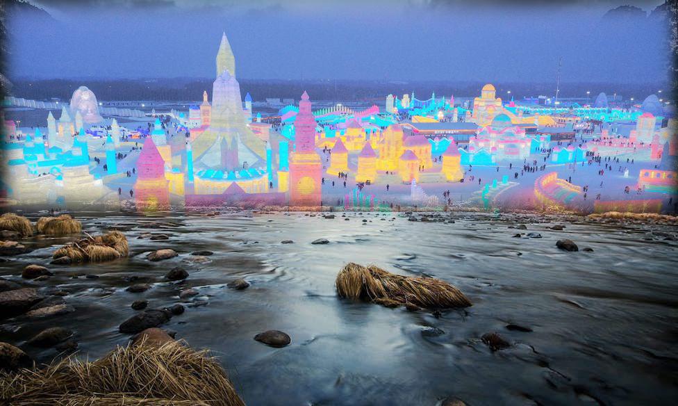
First, second, and third rows are from levels 0, 2, 4 of the laplacians. For bells and whistles, I then moved to color images. First I blended the oraple in color. Using a horizontal seam, I blended color images of Harbin and Yosemite. Because the horizon was at different levels, the result maybe is a bit more
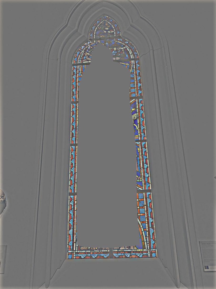
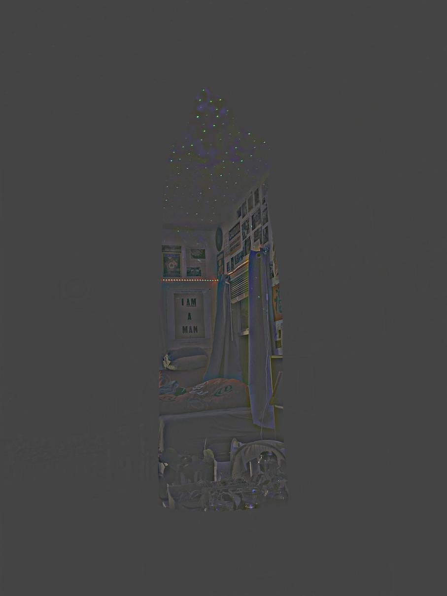
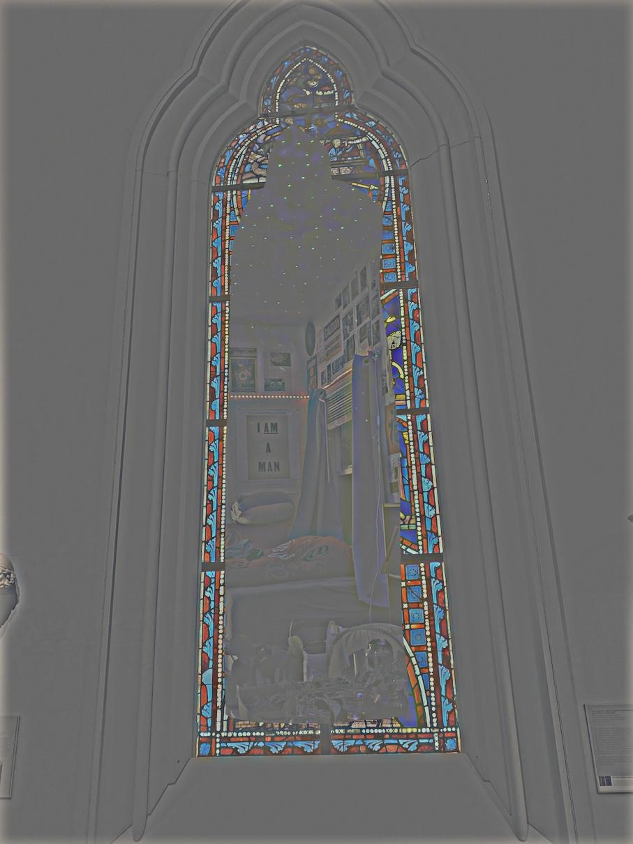
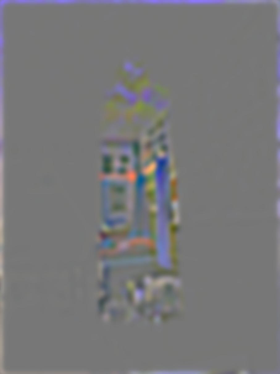
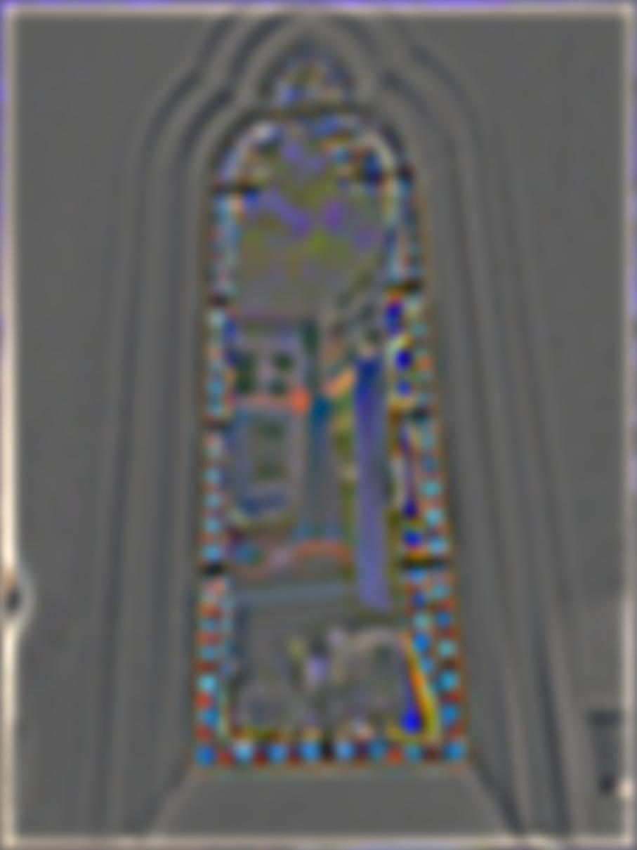
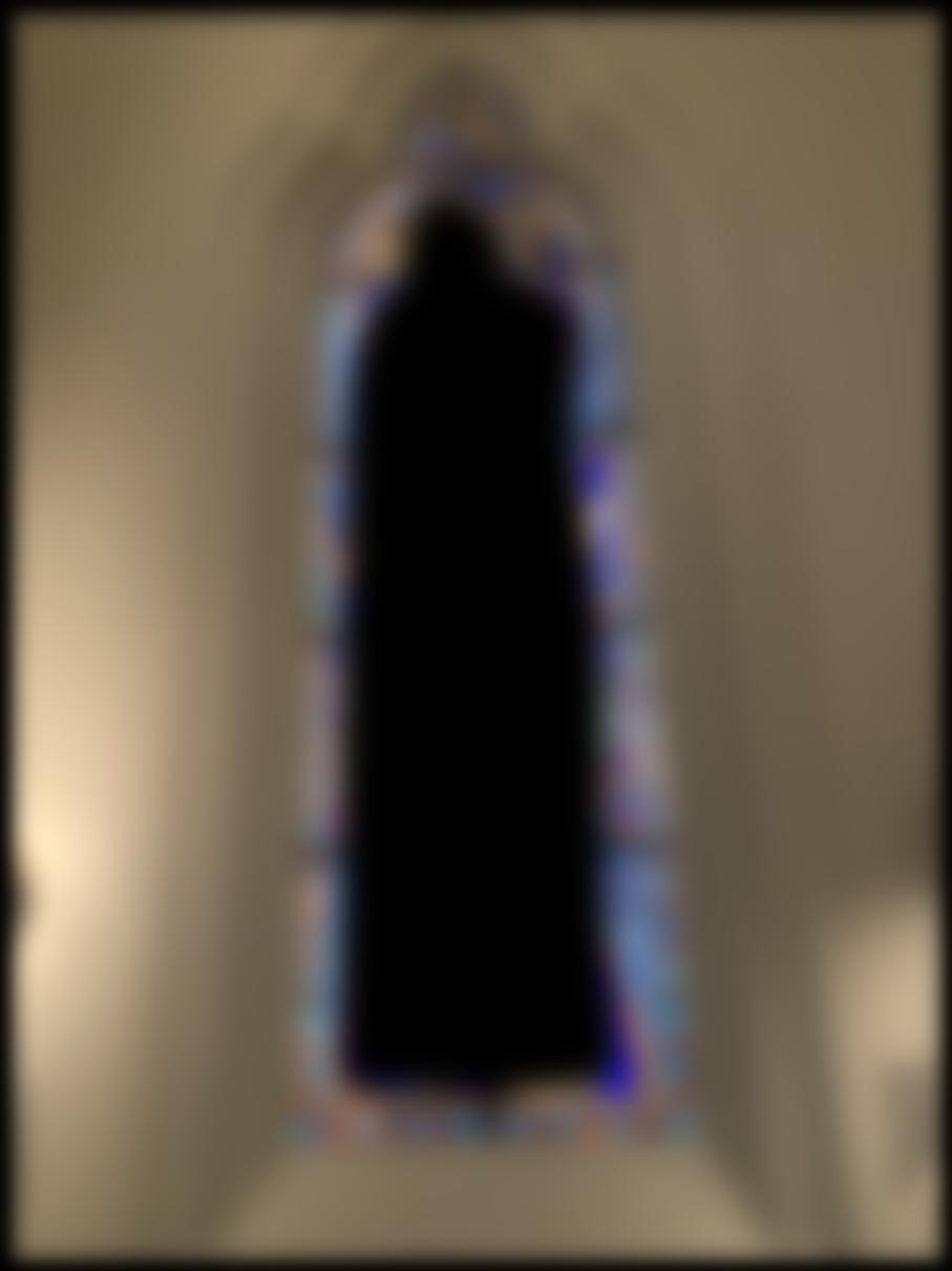
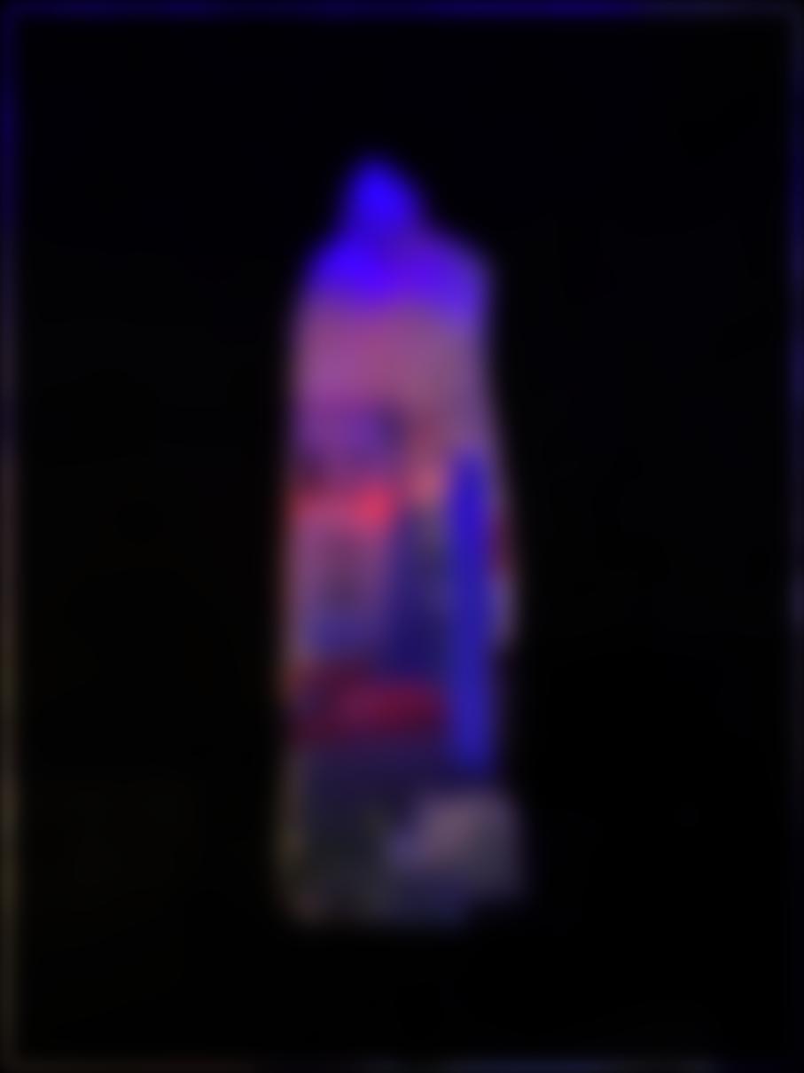
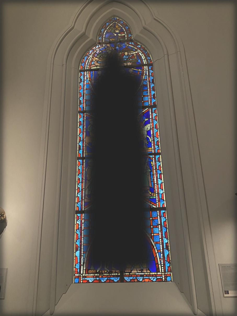
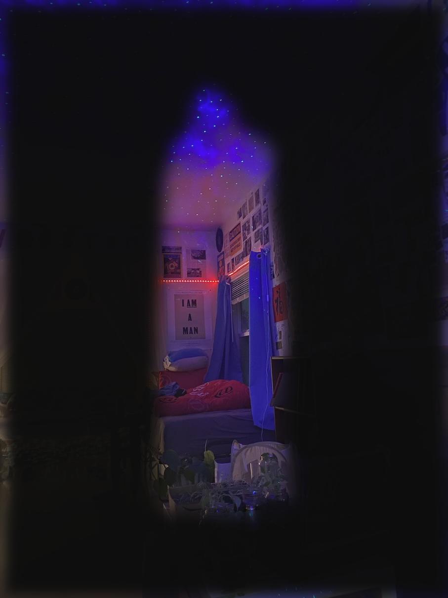
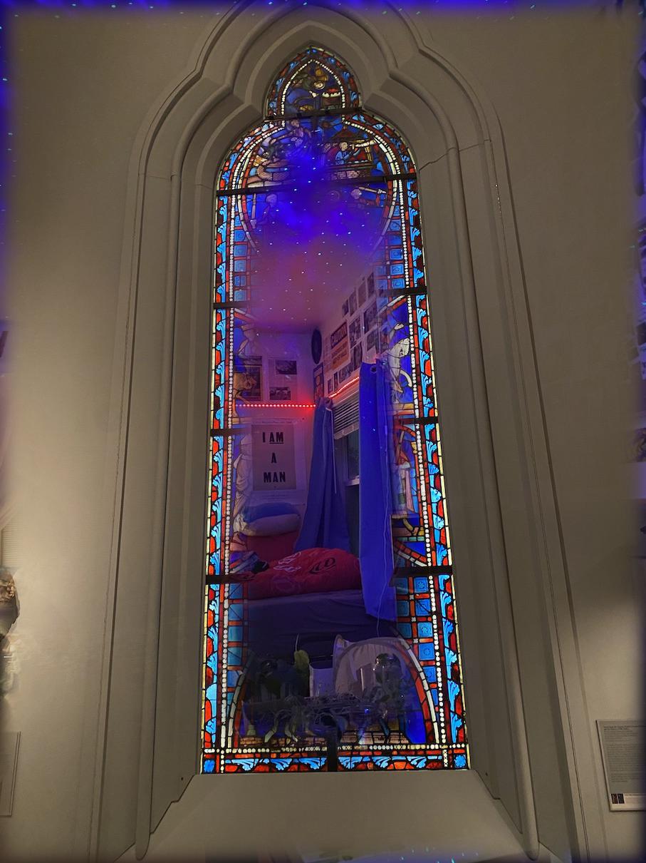
unnatural than I hoped, but still looks pretty cool. Then I used an irregular mask I created in photoshop, I blended a photo
of my room and a stained glass that I took a photo of in the Metropolitan
Museum to create a "portal".
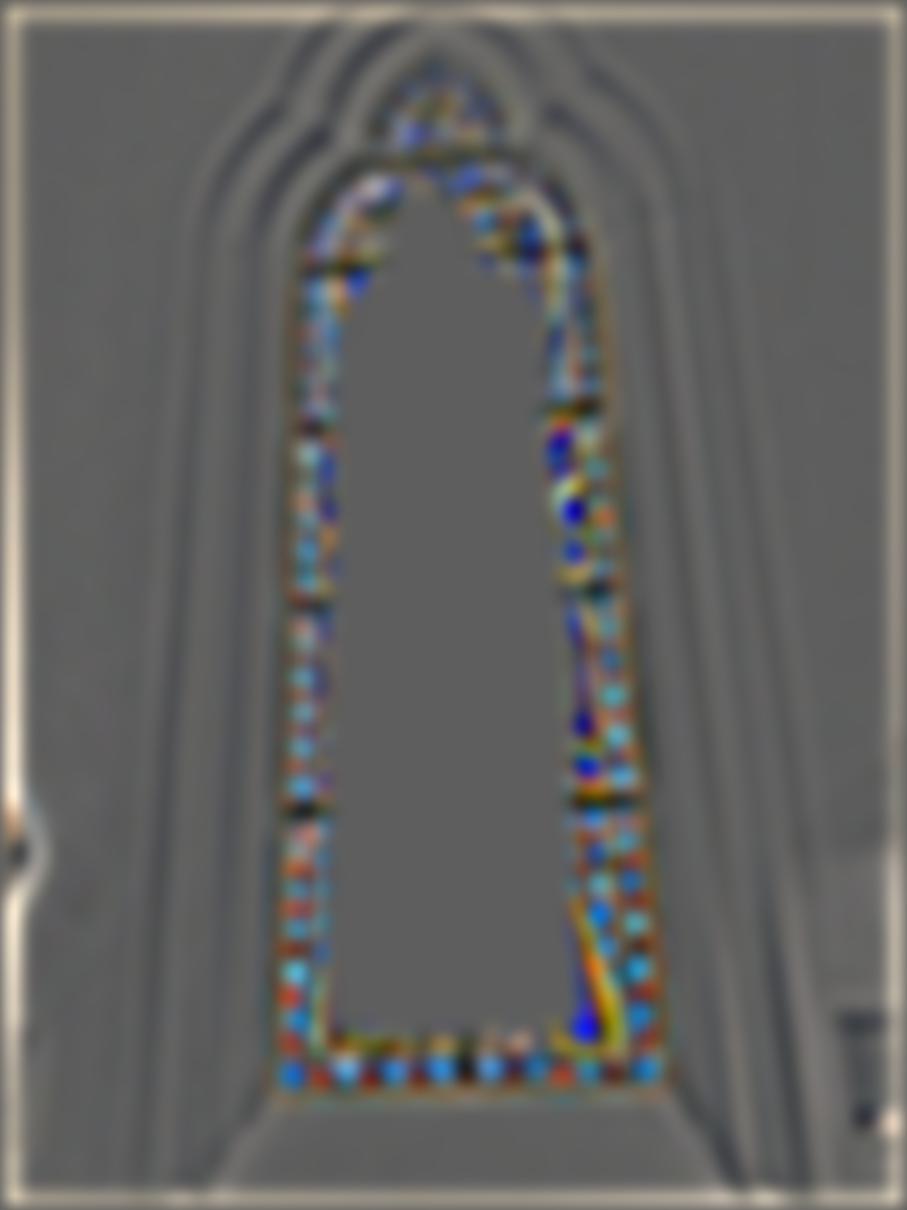
I compute a gaussian stack for the mask, and blend the laplacians at each
level with the filtered mask at that level.
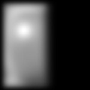
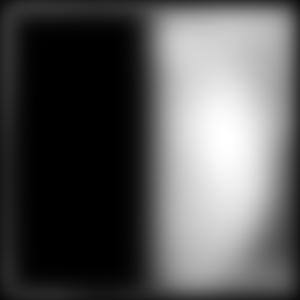
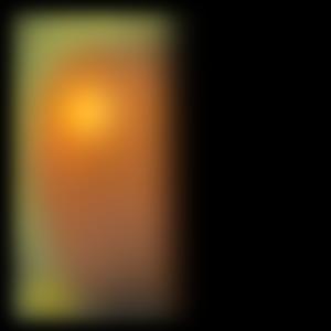
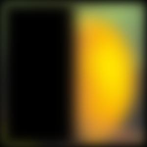
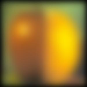
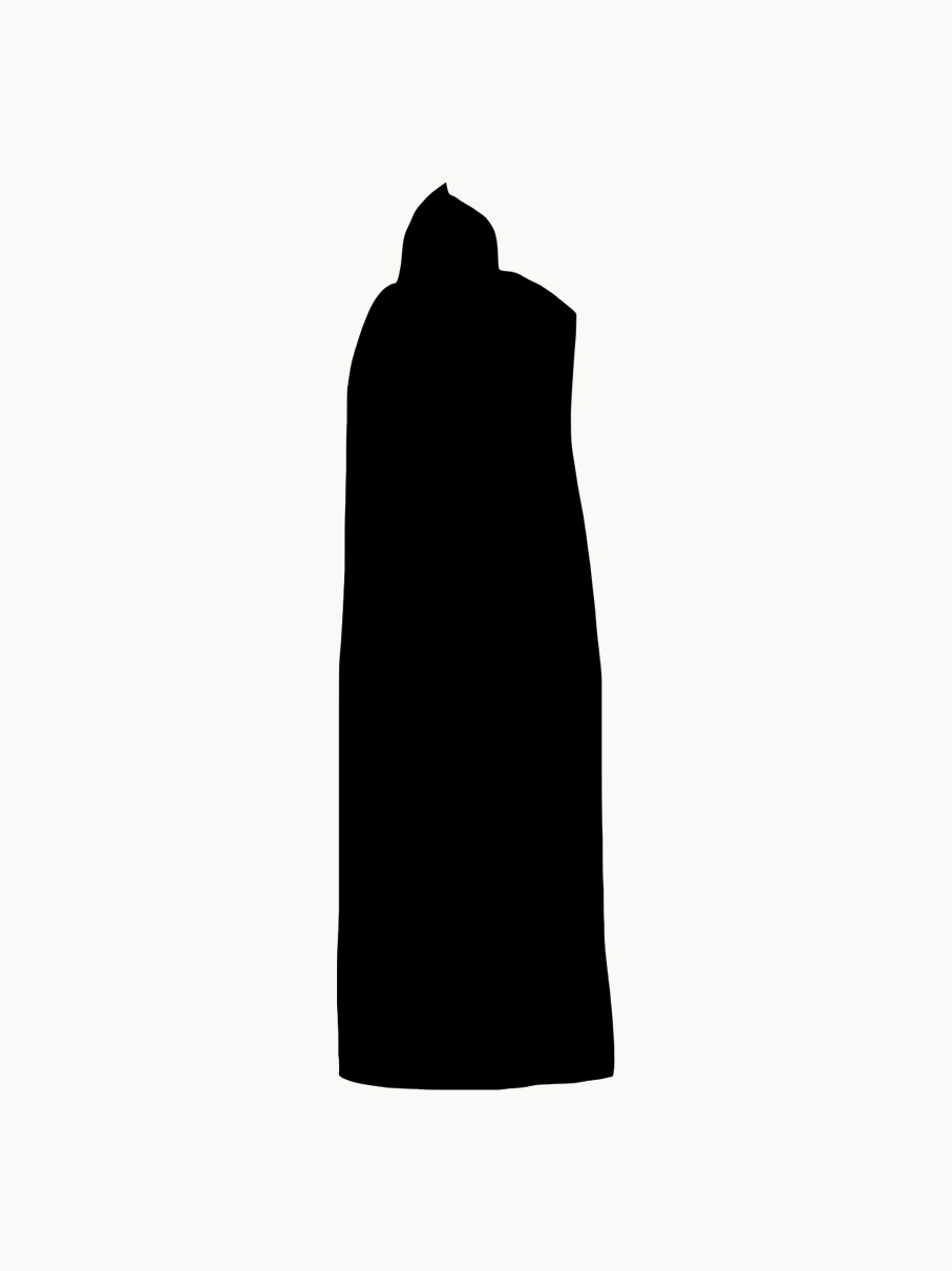
Here is the mask:
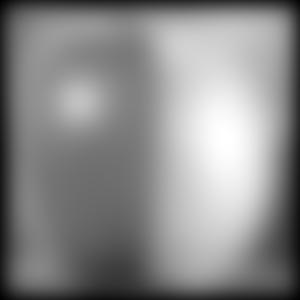
And here are the visualizations: